3.3 Global Constraints

3.3.1 Alldifferent constraints

Alldifferent constraint ensures that all FDVs from a given list have different values assigned. This constraint uses a simple consistency technique that removes a value, which is assigned to a given FDV from the domains of the other FDVs.

For example, a constraint

enforces that the FDVs a, b, and c have different values.

Alldifferent constraint is provided as three different implementations. Constraint Alldifferent uses a simple implementation described above, i.e., if the domain of a finite domain variable gets assigned a value, the propagation algorithm will remove this value from the other variables. Constraint Alldiff implements this basic pruning method and, in addition, bounds consistency [13]. Finally, constraint Alldistinct implements a generalized arc consistency as proposed by Régin [14].

The example below illustrates the difference in constraints pruning power for Alldifferent and Alldiff constraints. Assume the following variables:

The constraints will produce the following results after consistency enforcement.

and

Alldistinct constraint will prune domains of variables a, b and c in the same way as Alldiff constraints but, in addition, it can remove single inconsistent values as illustrated below. Assume the following domains for a, b and c.

The constraints will produce the following results after consistency enforcement.

3.3.2 Circuit constraint

Circuit constraint tries to enforce that FDVs which represent a directed graph will create a Hamiltonian circuit. The graph is represented by the FDV domains in the following way. Nodes of the graph are numbered from 1 to N. Each position in the list defines a node number. Each FDV domain represents a direct successors of this node. For example, if FDV x at position 2 in the list has domain 1, 3, 4 then nodes 1, 3 and 4 are successors of node x. Finally, if the i’th FDV of the list has value j then there is an arc from i to j.

For example, the constraint

can find a Hamiltonian circuit [2, 3, 1], meaning that node 1 is connected to 2, 2 to 3 and finally, 3 to 1.

3.3.3 Subcircuit constraint

Subcircuit constraint tries to enforce that FDVs which represent a directed graph will create a subcircuit. The graph is represented by the FDV domains in the same way as for the Circuit constraint. The result defines a subcircuit represented by values assigned to the FDVs. Nodes that do not belong to a subcircuit have the value pointing to itself.

For example, the constraint

can find a circuit [2, 1, 3], meaning that node 1 is connected to 2 and 2 to 1 while node 3 is not in the subcircuit and has a value 3.

All solutions to this constraint are [1, 2, 3], [1, 3, 2], [2, 1, 3], [2, 3, 1], [3, 1, 2], [3, 2, 1], where the first solution represents a solution with no subsircuits and subseqent solutions define found subcrircuits.

3.3.4 Element constraint

Element constraint of the form Element(I, List, V ) enforces a finite relation between I and V , V = List[I]. The vector of values, List, defines this finite relation. For example, the constraint

imposes the relation on the index variable i :: {1..3}, and the value variable v. The initial domain of v will be pruned to v :: {3,10,44} after the intial consistency execution of this Element constraint. The change of one FDV propagates to another FDV. Imposing the constraint V < 44 results in change of I :: {1,3}.

This constraint can be used, for example, to define discrete cost functions of one variable or a relation between task delay and its implementation resources. The constraint is simply implemented as a program which finds values allowed both for the first FDV and third FDV and updating them respectively.

There are also two other versions of element constraint that implement a version of bounds consistency, ElementIntegerFast and ElementVariableFast. This constraints make faster computations but may not remove all inconsistent values.

3.3.5 Distance constraint

Distance constraint computes the absolute value between two FDVs. The result is another FDV, i.e., d = |x - y|.

The example below

produces result a::1..6, b::2..4, c::0..2 since a must be pruned to have distance lower than three.

3.3.6 Cumulative constraint

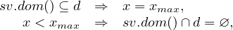
Cumulative constraint was originally introduced to specify the requirements on tasks which needed to be scheduled on a number of resources. It expresses the fact that at any time instant the total use of these resources for the tasks does not exceed a given limit. It has, in our implementation, four parameters: a list of tasks’ starts O_i, a list of tasks’ durations D_i, a list of amount of resources AR_i required by each task, and the upper limit of the amount of used resources Limit. All parameters can be either domain variables or integers. The constraint is specified as follows.

Formally, it enforces the following constraint:

(3.1)

In the above formulation, min and max stand for the minimum and the maximum values in the domain of each FDV respectively. The constraints ensures that at each time point, t, between the start of the first task (task selected by min(O_i)) and the end of the last task (task selected by max(O_i + D_i)) the cumulative resource use by all tasks, k, running at this time point is not greater than the available resource limit. This is shown in Fig 3.1.

JaCoP additionally requires that there exist at least one time point where the number of used resources is equal to Limit, i.e.

(3.2)

There is a version of Cumulative that only requires that the sum of AR_k ≤ Limit and it is defined with addtional flag as follows. In this constraint, first two flags specify to make propagation based on edge finding algorithm and profile while the last flag informs the solver to not apply reuirement 3.2.

3.3.7 Diff2 constraint

Diff2 constraint takes as an argument a list of 2-dimensional rectangles and assures that for each pair i,j (i≠j) of such rectangles, there exists at least one dimension k where i is after j or j is after i, i.e., the rectangles do not overlap. The rectangle is defined by a 4-tuple [O₁, O₂, L₁, L₂], where O_i and L_i are respectively called the origin and the length in i-th dimension. The diff2 constraint is specified as follows.

The Diff2 constraint can be used to express requirements for packing and placement problems as well as define constraints for scheduling and resource assignment.

This constraint uses two different propagators. The first one tries to narrow O_i and L_i FDV’s of each rectangle so that rectangles do not overlap. The second one is similar to the cumulative profile propagator but it is applied in both directions (in 2-dimensional space) for all rectangles. In addition, the constraint checks whether there is enough space to place all rectangles in the limits defined by each rectangle FDV’s domains.

3.3.8 Min, Max and ArgMin, ArgMax constraints

These constraints enforce that a given FDV is minimal or maximal of all variables present on a defined list of FDVs.

For example, a constraint

will constraint FDV min to a minimal value of variables a, b and c.

NOTE! The position for parameters in constraints Min and Max is changed comparing to previous versions (i.e., parameters are swapped).

The related constraints ArgMinArgMax find an index of the minimal and maximal element respectively. In the standard version the first position of the minimal or maximal element is constrained. Indexing starts from 1 if the parameter offset is not used.

3.3.9 Sum, SumWeight, SumWeightDom and Linear constraints

These constraints enforce that a sum of elements of FDVs’ vector is equal to a given FDV sum, that is x₁ + x₂ + + x_n = sum. The weighted sum is provided by the constraint SumWeight and imposes the following constraint w₁ ⋅x₁ + w₂ ⋅x₂ + + w_n ⋅x_n = sum. The above mentioned constraints use bounds consistency while constraint SumWeightDom uses domain consistency.

For example, the constraint

will constraint FDV sum to the sum of a, b and c.

Constraints Sum, SumWeight and SumWeightDom extend class Constraint while constraint Linear is a primitive constraint. It means that it can be an argument in other constraints, such as Reified, conditional and logical constraints. It is defined as w₁ ⋅ x₁ + w₂ ⋅ x₂ + + w_n ⋅ x_n ℜ sum, where sum is an integer constant and ℜ∈{<,≤,>,≥,=,≠}.

For example, the linear constraint can be used in reification, as follows.

Moreover there exist primitive constraints LinearInt and SumInt that implement pruning methods for large linear constraints presented in [6]. There exist also constraint LinearIntDom that implements domain consistency for linear constraint. This constraint has exponential complexity in worst case and need to be used carefully.

3.3.10 ExtensionalSupport and ExtensionalConflict constraints

There exist several implementation of these constraint distinguished by their suffixes. The base implementation with suffix VA tries to balance the usage of memory versus time efficiency. ExtensionalSupportMDD uses multi-valued decision diagram (MDD) as internal representation and algorithms proposed in [2] while ExtensionalSupportSTR uses simple tabular reduction (STR) and the method proposed in [10].

Extensional support and extensional conflict constraints define relations between n FDVs. Both constraints are defined by a vector of n FDVs and a vector of n-tuples of integer values. The n-tuples define the relation between variables defined in the first vector.

The tuples of extensional support constraint define all combinations of values that can be assigned to variables specified in the vector of FDVs. Extensional conflict, on the other hand specifies the combinations of values that are not allowed in any assignment to variables.

The example below specifies the XOR logical relation of the form a ⊕ b = c using both constraints.

3.3.11 Assignment constraint

Assignment constraint implements the following relation between two vectors of FDVs X_i = j ∧ Y _j = i.

For example, the constraint

produces the following assignment to FDVs when x[1] = 3.

The constraint has possibility to define the minimal index for vectors of FDVs. Therefore constraint Assignment(x, y, 1) will index variables from 1 instead of default value 0.

3.3.12 Count constraint

Count constraint counts number of occurrences of value Val on the list List in FDV Var.

For example, the constraint

produces Var :: {1..2}.

If variable Var will be constrained to 1 then JaCoP will produce produces List_1 :: {0..1} .

NOTE! The position for parameters in constraint Count is changed comparing to previous versions.

3.3.13 Values constraint

Values constraint takes as arguments a list of variables and a counting variable. It counts a number of different values on the list of variables in the counting variable. For example, consider the following code.

Constraint Values will remove value 2 from variable x3 to assure that are only two different values (1 and 3) on the list of variables as specified by variable count.

NOTE! The position for parameters in constraint Values is changed comparing to previous versions.

3.3.14 Global cardinality constraint (GCC)

Global cardinality constraint (GCC) is defined using two lists of variables. The first list is the value list and the second list is the counter list. The constraint counts number of occurrences of different values in the variables from the value list. The counter list is used to counter occurrences of a specific value. It can also specify the number of allowed occurrences of a specific value on the value list. Variables on the counter list are assigned to values as follows. The lowest value in the domain of all variables from the value list is counted by the first variable on the counters list. The next value (+1) is counted by the next variable and so on.

For example, the following code counts number of values -1, 0, 1 and 2 on value list x. The values are counted using counter list y using the following mapping. -1 is counted in y0, 0 is counted in y1, 1 is counted in y2 and 2 is counted in y3.

The GCC constraint will allow only the following five combinations of x variables [x0=-1, x1=0, x2=2], [x0=-1, x1=1, x2=2], [x0=-1, x1=2, x2=0], [x0=-1, x1=2, x2=1], and [x0=-1, x1=2, x2=2].

3.3.15 Among and AmongVar

Among constraint is specified using three parameters. The first parameter is the value list, the second one is a set of values specified as IntervalDomain, and finally the third parameter, the counter, counts the number of variables from the value list that get assigned values from the set of values. The constraint assures that exactly the number of variables defined by count variable is equal to one value from the set of values.

The following example constraints that either 2 or 4 variables from value list numbers are equal either 1 or 3. There exist 2880 such assignments.

AmongVar constraint is a generalization of Among constraint. Instead of specifying a set of values it uses a list of variables as the second parameter. It counts how many variables from the value list are equal to at least one variable from list of variables (second parameter).

The example below specifies the same conditions as the Among constraint in the above example.

3.3.16 Regular constraint

Regular constraint accepts only the assignment to variables that are accepted by an automaton. The automaton is specified as the first parameter of this constraint and a list of variable is the second parameter. This constraint implements a polynomial algorithm to establish GAC.

The automaton is specified by its states and transitions. There are three types of states: initial state, intermediate states, and final states. Each transition has associated domain containing all values which can trigger this transition. Values assigned to transitions must be present in the domains of assigned constraint variable. Each value may cause firing of the related transition. The automaton eventually reaches a final state after taking the last transition as specified by the value of the last variable.

Each state can be assigned a level by topologically sorting states of the automaton. The variables from the list (second parameters) are assigned to these levels. All states at the same level are assigned the same variable (see Figure 3.2). If necessary, the automaton, containing cycles, is unrolled to match a list of variables. Each transitions has assigned values that are allowed for a variable when the transition in the automaton is selected. This is specified as the interval domain.

The example below implements the automaton from Figure 3.2. This automaton defines condition for three variables to be different values 0, 1 or 2.

3.3.17 Knapsack constraint

Knapsack constraint specifies knapsack problem. This implementation¹ was inspired by the paper [8] and published in [11]. The major extensions of that paper are the following. The quantity variables do not have to be binary. The profit and capacity of the knapsacks do not have to be integers. In both cases, the constraint accepts any finite domain variable.

The constraint specify number of categories of items. Each item has a given weight and profit. Both weight and profit are specified as positive integers. The problem is to select a number of items in each category to satisfy capacity constraint, i.e. the total weight must be in the limits specified by the capacity variable. Each such solution is then characterized by a given profit. It is defined in JaCoP as follows.

It can be formalize using the following constraints.

(3.3) (3.4) (3.5)

3.3.18 Geost constraint

Geost is a geometrical constraint, which means that it applies to geometrical objects. It models placement problems under geometrical constraints, such as non overlapping constraints. Geost consistency algorithm was proposed by Beldiceanu et al [15]. The implementation of Geost in JaCoP is a result of a master thesis by Marc-Olivier Fleury.

In order to describe the constraint, we will introduce several definitions and relate them to JaCoP implementation.

Shifted box is defined in JaCoP using class DBox. For example, a two dimensional shifted box starting at coordinates (0,0) and having length 2 in first dimension and 1 in second direction is specified as follows.

In JaCoP, we can define n shapes as collection of shifted boxes. Shape identifiers start at 0 and must be assigned consecutive integers. Therefore we have shapes with identifiers in interval 0..n-1. The following JaCoP example defines a shape with identifier 0, consisting of three sboxs, depicted in Figure 3.4.

An object in JaCoP is defined by class GeostObject. It specifies basically all parameters of an object. An example below specifies object 0 that can take shapes 0, 1, 2 and 3. The object can be placed using coordinates (X_o1, Y_o1). The object is present during time 2 to 14.

Note that since object shapes are defined in terms of collections of shifted boxes, and since shifted boxes have a fixed size, Geost is not suited to solve problems in which object sizes can vary. Polymorphism provides some flexibility (shape variable having multiple values in their domain), but it is essentially intended to allow the modeling of objects that can take a small amount of different shapes. Typically objects that can be rotated. The duration of an object can be useful in cases where objects have variable sizes, because it is a variable, which means that some more flexibility is available. However, this feature is only available for one dimension. These restrictions are design choices made by the authors of Geost, probably because it fits well their primary field of application, which consists in packing goods in trucks. Using fixed sized shapes is also useful because it allows more deductions concerning possible placements.

When all shapes and objects are defined it is possible to specify geometrical constraints that must be fulfilled when placing these objects. Implemented geometrical constraints include in-area and non-overlapping constraints. In-area constraint enforces that objects have to lie inside a given k-dimensional sbox. Non-overlapping constraints require that no two objects can overlap.

The code below specifies two geometrical constraint, non-overlapping and in-area. They are specified by classes NonOverlapping and InArea. It must be noted that non-overlapping constraint in the code below specifies that all objects must not overlap in its two dimensions and time dimension (the time dimension is implemented as one additional dimension and therefore we specify dimensions 0, 1 and 2). In-area constraint requires that all object must be included in the sbox of dimensions 5x4.

Finally, the Geost constraint is imposed using the following code.

3.3.19 NetworkFlow constraint

NetworkFlow constraint defines a minimum-cost network flow problem. An instance of this problem is defined on a directed graph by a tuple (N,A,l,u,c,b), where

• N is the set of nodes,
• A is the set of directed arcs,
• l : A → ℤ_≥0 is the lower capacity function on the arcs,
• u : A → ℤ_≥0 is the upper capacity function on the arcs,
• c : A → ℤ is the flow cost-per-unit function on the arcs,
• b : N → ℤ is the node mass balance function on the nodes.

A flow is a function x : A → ℤ_≥0. The minimum-cost flow problem asks to find a flow that satisfies all arc capacity and node balance conditions, while minimizing total cost. It can be stated as follows:

The network is built with NetworkBuilder class using node, defined by class org.jacop.net.Node and arcs. Each node is defined by its name and node mass balance b. For example, node A with balance 0 is defined using network net as follows.

Source node producing flow of capacity 5 and sink node consuming flow of capacity 5 are defined using similar constructs but different value of node mass balance, as indicated below.

Arc of the network are defined always between two nodes. They define connection between given nodes, the lower and upper capacity values assigned to the arc (values l and u) as well as the flow cost-per-unit function on the arc (value c). This can be defined using different methods with either integers or finite domain variables. For example, an arc from source to node A with l = 0 and u = 5 and c = 3 can be defined as follows.

or

It can be noted, that cost-per-unit value can also be defined as a finite domain variable.

The constraint has also the flow cost, defined as z(x) in 3.6. It is defined as follows.

Note that the NetworkFlow only ensures that cost z(x) ≤ Z^max, where z(x) is the total cost of the flow (see equation (3.6)). In our code it is defined as variable cost.

The constraint is finally posed using the following method.

For example, Figure 3.5 presents the code for network flow problem depicted in Figure 3.6. The minimal flow, found by the solver, is 10 that is indicated in the figure.

Network builder has a special attribute handlerList that makes it possible to specify structural rules connected to the network. Each structural rule must implement VarHandler interface, which allows network flow constraint to cooperate with the structural rule. An important, already implemented rule, is available in the class DomainStructure. It specifies, for each structural variable sv, a list of arcs that the structural rule influence. This structural rule makes it possible to enforce minimum or maximum amount of flow on a given arc depending on the relationship between the domain of variable sv and domain d, specified within a structural rule. The domain of variable sv and domain d do not intersect if and only if the flow on a given arc is minimal as specified by initial value x.min(), denoted as x_min. Moreover, the domain of varibale sv is contained within domain d if and only if the actual flow on a given arc is maximal as specified by initial value x.max(), denoted as x_max. It is enforced by the following rules.

(3.9)

(3.10)

For example, creation of structural rule for arc between node source and B will enforce that this arc will have maximal flow if variable s is zero and minimal flow otherwise. The rule works also in the other direction, i.e. if the flow will be maximal variable s=0 and if the flow will be minimal this variable will be 1.

SoftAlldifferent constraint as well as SoftGCC constraint use DomainStructure rules to enforce flow from variable nodes to value nodes according the actual domain/value of variables represented by variable nodes. It is crucial functionality for the implementation of those soft global constraints.

3.3.20 Binpacking

Binpacking constraint defines a problem of packing bins with the specified items of a given size. Each bin has a defined load. The constraint is defined as follows.

where item means the bin number assigned to item at position i, load defines load of bin i as finite domain variable (min and max load) and size defines items i size.

It can be formalize using the following formulation.

(3.11)

The binpacking constraint implements methods and algorithms proposed in [17].