__________________________________________________________________
Version 4.9, September 19, 2022
Copyright ©2002–2022 Krzysztof Kuchcinski and Radosław Szymanek. All rights reserved.
JaCoP library provides constraint programming paradigm implemented in Java. It provides primitives to define finite domain (FD) variables, constraints and search methods. The user should be familiar with constraint (logic) programming (CLP) to be able to use this library. A good introduction to CLP can be found, for example, in [18].
JaCoP library provides most commonly used primitive constraints, such as equality, inequality as well as logical, reified and conditional constraints. It contains also number of global constraints. These constraints can be found in most commercial CP systems [4, 25, 6, 22]. Finally, JaCoP defines also decomposable constraints, i.e., constraints that are defined using other constraints and possibly auxiliary variables.
JaCoP library can be used by providing it as a JAR file or by specifying access to a directory containing all JaCoP classes. An example how program Main.java, which uses JaCoP, can be compiled and executed in the Linux like environment is provided below.
   javac -classpath .:path_to_JaCoP Main.java
   java -classpath .:path_to_JaCoP Main
or
   javac -classpath .:JaCoP.jar Main.java
   java -classpath .:JaCoP.jar Main
Alternatively one can specify the class path variable.
In Java application which uses JaCoP it is required to specify import statements for all used classes from JaCoP library. An example of the import statements that import the whole subpackages of JaCoP at once is shown below.
   import org.jacop.core.*;
   import org.jacop.constraints.*;
   import org.jacop.search.*;
Obviously, different Java IDE (Eclipse, IntelliJ, NetBeans, etc.) and pure Java build tools (e.g., Ant, Maven) can be used for JaCoP based application development.
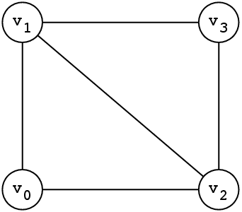
Consider the problem of graph coloring as depicted in Fig. 1.1. Below, we provide a simplistic program with hard-coded constraints and specification of the search method to solve this particular graph coloring problem.
import org.jacop.core.*;

import org.jacop.constraints.*;

import org.jacop.search.*;


public class Main {


    static Main m = new Main ();


    public static void main (String[] args) {

        Store store = new Store();  // define FD store

        int size = 4;

        // define finite domain variables

        IntVar[] v = new IntVar[size];

        for (int i=0; i<size; i++)

            v[i] = new IntVar(store, "v"+i, 1, size);

        // define constraints

        store.impose( new XneqY(v[0], v[1]) );

        store.impose( new XneqY(v[0], v[2]) );

        store.impose( new XneqY(v[1], v[2]) );

        store.impose( new XneqY(v[1], v[3]) );

        store.impose( new XneqY(v[2], v[3]) );


        // search for a solution and print results

        Search<IntVar> search = new DepthFirstSearch<IntVar>();

        SelectChoicePoint<IntVar> select =

            new InputOrderSelect<IntVar>(store, v,

                                         new IndomainMin<IntVar>());

        boolean result = search.labeling(store, select);


        if ( result )

            System.out.println("Solution: " + v[0]+", "+v[1] +", "+

                                              v[2] +", "+v[3]);

        else

            System.out.println("*** No");

    }

}
This program produces the following output indicating that vertices v0, v1 and v3 get different colors (1, 2 and 3 respectively), while vertex v3 is assigned color number 1.
Solution: v0=1, v1=2, v2=3, v3=1
The problem is specified with the help of variables (FDVs) and constraints over these variables. JaCoP support both finite domain variables (integer variables) and set variables. Both variables and constraints are stored in the store (Store). The store has to be created before variables and constraints. Typically, it is created using the following statement.
Store store = new Store();
The store has large number of responsibilities. In short, it knits together all components required to model and solve the problem using JaCoP (CP methodology). One often abused functionality is printing method. The store has redefined the method toString(), but use it with care as printing large stores can be a very slow/memory consuming process.
In the next sections we will describe how to define FDVs and constraints.
Variable X :: 1..100 is specified in JaCoP using the following general statement (assuming that we have defined store with name store). Clerly, we required to have created store before we can create variables as any constructor for variable will require providing the reference to store in which the variable is created.
IntVar x = new IntVar(store, "X", 1,100);
One can access the actual domain of FDV using the method dom(). The minimal and maximal values in the domain can be accessed using min() and max() methods respectively. The domain can contain “holes”. This type of the domain can be obtained by adding intervals to FDV domain, as provided below:
   IntVar x = new IntVar(store, "X", 1, 100);

   x.addDom(120, 160);
which represents a variable X with the domain 1..100 ∨ 120..160.
FDVs can be defined without specifying their identifiers. In this case, a system will use an identifier that starts with “_” followed by a generated unique sequential number of this variable, for example “_123”. This is illustrated by the following code snippet.
IntVar x = new IntVar(store, 1, 100);
FDVs can be printed using Java primitives since the method toString() is redefined for class Variable. The following code snippet will first create a variable with the domain containing values 1, 2, 14, 15, and 16.
   IntVar x = new IntVar(store, "x", 1, 2);

   x.addDom(14, 16);

   System.out.println(x);
The last line of code prints a variable, which produces the following output.
X::{1..2, 14..16}
One special variable class is a BooleanVariable. They have been added to JaCoP as they can be handled more efficiently than FDVs with multiple elements in their domain. They can be used as any other variable. However, some constraints may require BooleanVariables as parameters. An example of Boolean variable definition is shown below.
BooleanVar bv = new BooleanVar(s, "bv");
In the previous section, we have defined FDVs with domains without considering domain representation. JaCoP default domain (cllaed IntervalDomain) is represented as an ordered list of intervals. Each interval is represented by a pair of integers denoting the minimal and the maximal value. This representation makes it possible to define all possible finite domains of integers but it is not always computationally efficient. For some problems other representations might be more computationally efficient. Therefore, JaCoP also offers domain that is restricted to represent only one interval with its minimal and maximal value. This domain is called BoundDomain and can be used by a finite domain variable in a same way as interval domain. The only difference is that any attempt to remove values from inside the interval of this domain will have no effect.
The following code creates variable v with bound domain 1..10.
IntVar v = new IntVar(s, "v", new BoundDomain(1, 10) );
In JaCoP, there are three major types of constraints:
primitive constraints,
global constraints, and
decomposable constraints.
Primitive constraints and global constraints can be imposed using impose method, while decomposable constraints are imposed using imposeDecomposition method. An example that imposes a primitive constraint XneqY is defined below. Again, in order to impose a constraint a store object must be available.
store.impose( new XeqY(x1, x2));
Alternatively, one can define first a constraint and then impose it, as shown below.
   PrimitiveConstraint c = new XeqY(x1, x2);

   c.impose(store);
Both methods are equivalent.
The methods impose(constraint) and constraint.impose(store) often create additional data structures within the constraint store as well as constraint itself. Do note that constraint imposition does not involve checking if the constraint is consistent. Both methods of constraint imposition does not check whether the store remains consistent. If checking consistency is needed, the method imposeWithConsistency(constraint) should be used instead. This method throws FailException if the store is inconsistent. Note, that similar functionality can be achieved by calling the procedure store.consistency() explicitly (see section 6).
Constraints can have another constraints as their arguments. For example, reified constraints of the form X = Y ⇔ B can be defined in JaCoP as follows.
   IntVar x = new IntVar(store, "X", 1, 100);

   IntVar y = new IntVar(store, "Y", 1, 100);

   IntVar b = new IntVar(store, "B", 0, 1);

   store.impose( new Reified( new XeqY(x, y), b));
In a similar way disjunctive constraints can be imposed. For example, the disjunction of three constraints can be defined as follows.
   PrimitiveConstraint[] c = {c1, c2, c3};

   store.impose( new Or(c) );
or
   ArrayList<PrimitiveConstraint> c =

                          new ArrayList<PrimitiveConstraint>();

   c.add(c1); c.add(c2); c.add(c3);

   store.impose( new Or(c) );
Note, that disjunction and other similar constraints accept only primitive constraints as parameters.
After specification of the model consisting of variables and constraints, a search for a solution can be started. JaCoP offers a number of methods for doing this. It makes it possible to search for a single solution or to try to find a solution which minimizes/maximizes given cost function. This is achieved by using the depth-first-search together with constraint consistency enforcement.
The consistency check of all imposed constrains is achieved calling the following method from class Store.
boolean result = store.consistency();
When the procedure returns false then the store is in inconsistent state and no solution exists. The result true only indicates that inconsistency cannot be found. In other words, since the finite domain solver is not complete it does not automatically mean that the store is consistent.
To find a single solution the DepthFirstSearch method can be used. Since the search method is used both for finite domain variables and set variables it is recommended to specify the type of variables that are used in search. For finite domain variables, this type is usually <IntVar>. It is possible to not specify these information but it will generate compilation warnings if compilation option -Xlint:unchecked is used. A simple use of this method is shown below.
   IntVar[] vars;

   ...

   Search<IntVar> label = new DepthFirstSearch<IntVar>();

   SelectChoicePoint<IntVar> select =

            new InputOrderSelect<IntVar>(store,

                                   vars, new IndomainMin<IntVar>());

   boolean result = label.labeling(store, select);
The depth-first-search method requires the following information:
how to assign values for each FDV from its domain; this is defined by IndomainMin class that starts assignments from the minimal value in the domain first and later assigns successive values.
how to select FDV for an assignment from the array of FDVs (vars); this is decided explicitly here by InputOrderSelect class that selects FDVs using the specified order present in vars.
how to perform labeling; this is specified by DepthFirstSearch class that is an ordinary depth-first-search.
Different classes can be used to implement SelectChoicePoint interface. They are summarized in Appendix B. The following example uses SimpleSelect that selects variables using the size of their domains, i.e., variable with the smallest domain is selected first.
   IntVar[] vars;

   ...

   Search<IntVar> label = new DepthFirstSearch<IntVar>();

   SelectChoicePoint<IntVar> select =

                new SimpleSelect<IntVar>(vars,

                                         new SmallestDomain<IntVar>(),

                                         new IndomainMin<IntVar>());

   boolean result = label.labeling(store, select);
In some situations it is better to group FDVs and assign the values to them one after the other. JaCoP supports this by another variable selection method called SimpleMatrixSelect. An example of its use is shown below. This choice point selection heuristic works on two-dimensional lists of FDVs.
   IntVar[][] varArray;

   ...

   Search<IntVar> label = new DepthFirstSearch<IntVar>();

   SelectChoicePoint<IntVar> select =

                 new SimpleMatrixSelect<IntVar>(

                                       varArray,

                                       new SmallestMax<IntVar>(),

                                       new IndomainMin<IntVar>());

   boolean result = label.labeling(store, select);
The optimization requires specification of a cost function. The cost function is defined by a FDV that, with the help of attached (imposed) constraints, gets correct cost value. A typical minimization for defined constraints and a cost FDV is specified below.
   IntVar[] vars;

   IntVar cost;

   ...

   Search<IntVar> label = new DepthFirstSearch<IntVar>();

   SelectChoicePoint<IntVar> select = new SimpleSelect<IntVar>(vars,

                                       new SmallestDomain<IntVar>(),

                                       new IndomainMin<IntVar>());

   boolean result = label.labeling(store, select, cost);
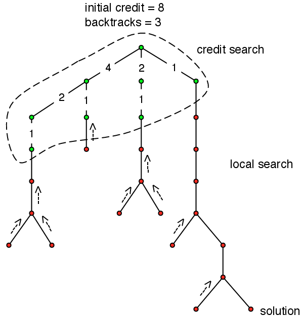
JaCoP offers number of different search heuristics based on depth-first-search. For example, credit search and limited discrepancy search. They are implemented using plug-in listeners that modify the standard depth-first-serch. For more details, see section 6.
All constraints must be posed with impose method when domains of all their variables are fully defined.
JaCoP offers a set of primitive constraints that include basic arithmetic operations (+,-,*,∕) as well as basic relations (=,≠,<,≤,>,≥). Subtraction is not provided explicitly, but since constraints define relations between variables, it canbe defined using addition. For detailed list of primitive constraint see appendix A.1.
Primitive constraints can be used as arguments in logical and conditional constraints.
Logical and conditional constraints use primitive constraints as arguments. JaCoP allows also specification of the reified, half-reified (implication) and if-then-elese (IfThen, IfThenElse, Conditional) constraints. For detailed list of these constraints see appendix A.4.
Alldifferent constraint ensures that all FDVs from a given list have different values assigned. This constraint uses a simple consistency technique that removes a value, which is assigned to a given FDV from the domains of the other FDVs.
For example, a constraint
   IntVar a = new IntVar(store, "a", 1, 3);

   IntVar b = new IntVar(store, "b", 1, 3);

   IntVar c = new IntVar(store, "c", 1, 3);

   IntVar[] v = {a, b, c};

   Constraint ctr = new Alldifferent(v);

   store.impose(ctr);
enforces that the FDVs a, b, and c have different values.
Alldifferent constraint is provided as three different implementations. Constraint Alldifferent uses a simple implementation described above, i.e., if the domain of a finite domain variable gets assigned a value, the propagation algorithm will remove this value from the other variables. Constraint Alldiff implements this basic pruning method and, in addition, bounds consistency [16]. Finally, constraint Alldistinct implements a generalized arc consistency as proposed by Régin [20].
The example below illustrates the difference in constraints pruning power for Alldifferent and Alldiff constraints. Assume the following variables:
   IntVar a = new IntVar(store, "a", 2, 3);

   IntVar b = new IntVar(store, "b", 2, 3);

   IntVar c = new IntVar(store, "c", 1, 3);

   IntVar[] v = {a, b, c};
The constraints will produce the following results after consistency enforcement.
   store.impose( new Alldifferent(v) );


   a :: {2..3}, b :: {2..3}, c :: {1..3}
and
   store.impose( new Alldiff(v) );


   a :: {2..3}, b :: {2..3}, c = 1
Alldistinct constraint will prune domains of variables a, b and c in the same way as Alldiff constraints but, in addition, it can remove single inconsistent values as illustrated below. Assume the following domains for a, b and c.
a :: {1,3}, b :: {1,3}, c :: {1..3}
The constraints will produce the following results after consistency enforcement.
   store.impose( new Alldistinct(v) );


   a :: {1,3}, b :: {1,3}, c = 2
Circuit constraint tries to enforce that FDVs which represent a directed graph will create a Hamiltonian circuit. The graph is represented by the FDV domains in the following way. Nodes of the graph are numbered from 1 to N. Each position in the list defines a node number. Each FDV domain represents a direct successors of this node. For example, if FDV x at position 2 in the list has domain 1, 3, 4 then nodes 1, 3 and 4 are successors of node x. Finally, if the i’th FDV of the list has value j then there is an arc from i to j.
For example, the constraint
   IntVar a = new IntVar(store, "a", 1, 3);

   IntVar b = new IntVar(store, "b", 1, 3);

   IntVar c = new IntVar(store, "c", 1, 3);

   IntVar[] v = {a, b, c};

   Constraint ctr = new Circuit(store, v);

   store.impose(ctr);
can find a Hamiltonian circuit [2, 3, 1], meaning that node 1 is connected to 2, 2 to 3 and finally, 3 to 1.
Subcircuit constraint tries to enforce that FDVs which represent a directed graph will create a subcircuit. The graph is represented by the FDV domains in the same way as for the Circuit constraint. The result defines a subcircuit represented by values assigned to the FDVs. Nodes that do not belong to a subcircuit have the value pointing to itself.
For example, the constraint
   IntVar a = new IntVar(store, "a", 1, 3);

   IntVar b = new IntVar(store, "b", 1, 3);

   IntVar c = new IntVar(store, "c", 1, 3);

   IntVar[] v = {a, b, c};

   Constraint ctr = new Subcircuit(v);

   store.impose(ctr);
can find a circuit [2, 1, 3], meaning that node 1 is connected to 2 and 2 to 1 while node 3 is not in the subcircuit and has a value 3.
All solutions to this constraint are [1, 2, 3], [1, 3, 2], [2, 1, 3], [2, 3, 1], [3, 1, 2], [3, 2, 1], where the first solution represents a solution with no subsircuits and subseqent solutions define found subcrircuits.
Element constraint of the form Element(I, List, V ) enforces a finite relation between I and V , V = List[I]. The vector of values, List, defines this finite relation. For example, the constraint
   IntVar i = new IntVar(store, "i", 1, 3);

   IntVar v = new IntVar(store, "v", 1, 50);

   int[] el = {3, 44, 10};

   Constraint ctr = new Element(i, el, v);

   store.impose(ctr);
imposes the relation on the index variable i :: {1..3}, and the value variable v1 . The initial domain of v will be pruned to v :: {3,10,44} after the intial consistency execution of this Element constraint. The change of one FDV propagates to another FDV. Imposing the constraint V < 44 results in change of I :: {1,3}.
This constraint can be used, for example, to define discrete cost functions of one variable or a relation between task delay and its implementation resources. The constraint is simply implemented as a program which finds values allowed both for the first FDV and third FDV and updating them respectively.
There are also two other versions of element constraint that implement a version of bounds consistency, ElementIntegerFast and ElementVariableFast. This constraints make faster computations of consistency methods but may not remove all inconsistent values.
Distance constraint computes the absolute value between two FDVs. The result is another FDV, i.e., d = |x - y|.
The example below
   IntVar a = new IntVar(store, "a", 1, 10);

   IntVar b = new IntVar(store, "b", 2, 4);

   IntVar c = new IntVar(store, "c", 0, 2);

   Constraint ctr = new Distance(a, b, c);

   store.impose(ctr);
produces result a::1..6, b::2..4, c::0..2 since a must be pruned to have distance lower than three.
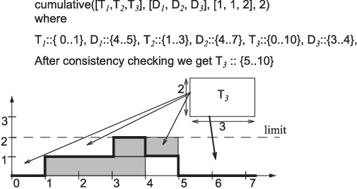
Cumulative constraint was originally introduced to specify the requirements on tasks which needed to be scheduled on a number of resources. It expresses the fact that at any time instant the total use of these resources for the tasks does not exceed a given limit. It has, in our implementation, four parameters: a list of tasks’ starts Oi, a list of tasks’ durations Di, a list of amount of resources ARi required by each task, and the upper limit of the amount of used resources Limit. All parameters can be either domain variables or integers. The constraint is specified as follows.
   IntVar[] o = {O1, ..., On};

   IntVar[] d = {D1, ..., Dn};

   IntVar[] r = {AR1, ..., ARn};

   IntVar Limit = new IntVar(Store, "limit", 0, 10);

   Constraint ctr = Cumulative(o, d, r, Limit)
Formally, it enforces the following constraint:
![∑
∀t ∈ [1 m≤iin≤n(Oi),1 m≤aix≤n(Oi + Di)] : ARk ≤ Limit
k:Ok≤t≤Ok+Dk](guideJaCoP0x.png) | (3.1) |
In the above formulation, min and max stand for the minimum and the maximum values in the domain of each FDV respectively. The constraints ensures that at each time point, t, between the start of the first task (task selected by min(Oi)) and the end of the last task (task selected by max(Oi + Di)) the cumulative resource use by all tasks, k, running at this time point is not greater than the available resource limit. This is shown in Fig 3.1.
JaCoP additionally requires that there exist at least one time point where the number of used resources is equal to Limit, i.e.
![∑
∃t ∈ [ min (Oi), max (Oi + Di)] : ARk = Limit
1≤i≤n 1≤i≤n k:Ok≤t≤Ok+Dk](guideJaCoP1x.png) | (3.2) |
There is a version of Cumulative that only requires that the sum of ARk ≤ Limit and it is defined with addtional flag as follows. In this constraint, first two flags specify to make propagation based on edge finding algorithm and profile while the last flag informs the solver to not apply reuirement 3.2.
   import org.jacop.constraints.Cumulative;

   Constraint ctr = Cumulative(o, d, r, Limit, true, true, false)
There exist also a newer implementation of cumulative constraints based on methods presented in [27, 26, 23]. There are three following cumulative constraints.
CumulativeBasic- does time-tabling propagation,
Cumulative- does time-tabling and edge finding propagation, and
CumulativeUnary- a specialized version for unary resources and it does in addition to time-tabling and edge finding (specialized for unary resource) propagations, not-first-not-last, detectable propagations.
All propagations, except time-tabling, are done on binary trees and have the following complexities, where n is the number of tasks and k is the number of distinct resource values for tasks. Edge finding O(k ⋅ n ⋅ logn), not-first-not-last, detectable and overload O(n ⋅ logn).
An example of using this implementation for Cumulative constraint is as follows.
   import org.jacop.constraints.cumulative.*;

   Constraint ctr = Cumulative(o, d, r, Limit)
Diffn constraint takes as an argument a list of 2-dimensional rectangles and assures that for each pair i,j (i≠j) of such rectangles, there exists at least one dimension k where i is after j or j is after i, i.e., the rectangles do not overlap. The rectangle is defined by a 4-tuple [O1, O2, L1, L2], where Oi and Li are respectively called the origin and the length in i-th dimension. The diffn constraint is specified as follows.
   import org.jacop.constraints.diffn.*;

   IntVar[][] rectangles = {{O11, O12, L11, L12}, ...,

                              {On1, On2, Ln1, Ln2}};

   Constraint ctr = new Diffn(rectangles)
Alternatively, the constraint can be specified using four lists of origins and lengths of rectangles.
   import org.jacop.constraints.diffn.*;

   IntVar[][] rectangles = {{O11, O21, ..., On1},

                            {O12, O22, ..., On2},

                            {L11, L21, ..., Ln1},

                            {L12, L22, ..., Ln2}};

   Constraint ctr = new Diffn(rectangles)
The special case for the constraint is when one length becomes zero. In this case, the constraint places zero-length rectangles between other rectangles, that is the zero-length rectangle cannot be placed anywhere. To make possible, the so called, non-strict placement, the constraint has possibility to use the last Boolean parameter equal false, meaning non-strict placement.
The Diffn constraint can be used to express requirements for packing and placement problems as well as define constraints for scheduling and resource assignment.
This constraint uses two different propagators. The first one tries to narrow Oi and Li FDV’s of each rectangle so that rectangles do not overlap. The second one is similar to the cumulative profile propagator but it is applied in both directions (in 2-dimensional space) for all rectangles. In addition, the constraint checks whether there is enough space to place all rectangles in the limits defined by each rectangle FDV’s domains.
Simplified version of the constraint that logically enforces no overlapping conditions on rectangles is available as well and is called Nooverlap. This constraint has weaker pruning but is faster for simple problems. DiffnDecomposed is the decomposed version of the constraint that combines no overlapping constraint with two cumulative constraints (in direction x ands y).
These constraints enforce that a given FDV is minimal or maximal of all variables present on a defined list of FDVs.
For example, a constraint
   IntVar a = new IntVar(Store, "a", 1, 3);

   IntVar b = new IntVar(Store, "b", 1, 3);

   IntVar c = new IntVar(Store, "c", 1, 3);

   IntVar min = new IntVar(Store, "min", 1, 3);

   IntVar[] v = {a, b, c};

   Constraint ctr = new Min(v, min);

   Store.impose(ctr);
will constraint FDV min to a minimal value of variables a, b and c.
NOTE! The position for parameters in constraints Min and Max is changed comparing to previous versions (i.e., parameters are swapped).
The related constraints ArgMinArgMax find an index of the minimal and maximal element respectively. In the standard version the first position of the minimal or maximal element is constrained. Indexing starts from 1 if the parameter offset is not used.
These constraints enforce a (wighted) sum of elements of FDVs’ vector
SumInt and SumBool constraint is defined as follows x1 + x2 +  + xn ℜ sum,
where all xi and sum are FDVs and ℜ∈{<,≤,>,≥,=,≠}. SumBool has additional
requirement that all FDVs must have domain 0..1.
+ xn ℜ sum,
where all xi and sum are FDVs and ℜ∈{<,≤,>,≥,=,≠}. SumBool has additional
requirement that all FDVs must have domain 0..1.
The weighted sum is provided by LinearInt constraint defined as follows
w1 ⋅x1 + w2 ⋅x2 +  + wn ⋅xn ℜ sum, where all wi and sum are integer constants, xi
are FDVs and ℜ∈{<,≤,>,≥,=,≠}. There exist also a constructor for LinearInt that
makes it possible to give sum as a FDV. In this case the constraint is transformed to its
normal form where FDV is added to the list of variables with weight -1 and the result is 0.
To define, for example, constraint w1 ⋅x1 + w2 ⋅x2 +
+ wn ⋅xn ℜ sum, where all wi and sum are integer constants, xi
are FDVs and ℜ∈{<,≤,>,≥,=,≠}. There exist also a constructor for LinearInt that
makes it possible to give sum as a FDV. In this case the constraint is transformed to its
normal form where FDV is added to the list of variables with weight -1 and the result is 0.
To define, for example, constraint w1 ⋅x1 + w2 ⋅x2 +  + wn ⋅xn = s where s is FDV, the
constraint will be internally transformed to w1 ⋅ x1 + w2 ⋅ x2 +
+ wn ⋅xn = s where s is FDV, the
constraint will be internally transformed to w1 ⋅ x1 + w2 ⋅ x2 +  + (-1) ⋅ s = 0.
For example, the constraint
   IntVar a = new IntVar(Store, "a", 1, 3);

   IntVar b = new IntVar(Store, "b", 1, 3);

   IntVar c = new IntVar(Store, "c", 1, 3);

   IntVar sum = new IntVar(Store, "sum", 1, 10);

   IntVar[] v = {a, b, c};

   Constraint ctr = new SumInt(v, "==", sum);

   Store.impose(ctr);
will constraint FDV sum to the sum of a, b and c.
Constraints SumInt, SumBool and LinearInt are primitive constraints. It means that they can be an argument in other constraints, such as Reified, conditional and logical constraints.
For example, the linear constraint can be used in reification, as follows.
   Store store = new Store();

   IntVar a = new IntVar(Store, "a", 1, 3);

   IntVar b = new IntVar(Store, "b", 1, 3);

   IntVar c = new IntVar(Store, "c", 1, 3);

   IntVar[] v = {a, b, c};

   PrimitiveConstraint ctr =

      new LinearInt(store, v, new int[] {2, 3, -1}, "<", 10);

   BooleanVar b = new BooleanVar(store);

   store.impose(new Reified(ctr), b);
Primitive constraints LinearInt and SumInt implement pruning methods for large linear constraints presented in [10]. There exist also constraint LinearIntDom that implements domain consistency for linear constraint. This constraint has exponential complexity in worst case and need to be used carefully. This constraint can be useful when computing an index from two dimensional array to a vector for element constraint.
Constraints Sum, SumWeight and SumWeightDom extend class Constraint and are deprecated.
There exist several implementation of these constraints. Table and SimpleTable constraints use compact-table algorithms proposed in [5]. ExtensionalSupport and ExtensionalConflict are distinguished by their suffixes. The base implementation with suffix VA tries to balance the usage of memory versus time efficiency. ExtensionalSupportMDD uses multi-valued decision diagram (MDD) as internal representation and algorithms proposed in [3] while ExtensionalSupportSTR uses simple tabular reduction (STR) and the method proposed in [15].
Extensional support, extensional conflict and table constraints define relations between n FDVs. All constraints are defined by a vector of n FDVs and a vector of n-tuples of integer values. The n-tuples define the relation between variables defined in the first vector.
The tuples of extensional support and table constraint define all combinations of values that can be assigned to variables specified in the vector of FDVs. Extensional conflict, on the other hand specifies the combinations of values that are not allowed in any assignment to variables.
The example below specifies the XOR logical relation of the form a ⊕ b = c using both constraints.
   IntVar a = new IntVar(store, "a", 0, 1);

   IntVar b = new IntVar(store, "b", 0, 1);

   IntVar c = new IntVar(store, "c", 0, 1);

   IntVar[] v = {a, b, c};

   // version with ExtensionalSupport constraint

   store.impose(new ExtensionalSupportVA(v,

                                         new int[][] {{0, 0, 0},

                                                      {0, 1, 1},

                                                      {1, 0, 1},

                                                      {1, 1, 0}}));
   // version with ExtensionalConflict constraint

   store.impose(new ExtensionalConflictVA(v,

                                          new int[][] {{0, 0, 1},

                                                       {0, 1, 0},

                                                       {1, 0, 0},

                                                       {1, 1, 1}}));
Assignment constraint implements the following relation between two vectors of FDVs Xi = j ∧ Y j = i.
For example, the constraint
   IntVar[] x = new IntVar[4];

   IntVar[] y = new IntVar[4];

   for (int i=0; i<4; i++) {

     x[i] = new IntVar(store, "x"+i, 0, 3);

     y[i] = new IntVar(store, "y"+i, 0, 3);

   }

   store.impose(new Assignment(x, y));
produces the following assignment to FDVs when x[1] = 3.
x0::{0..2}

x1=3

x2::{0..2}

x3::{0..2}

y0::{0, 2..3}

y1::{0, 2..3}

y2::{0, 2..3}

y3=1
The constraint has possibility to define the minimal index for vectors of FDVs. Therefore constraint Assignment(x, y, 1) will index variables from 1 instead of default value 0.
Count constraint counts number of occurrences of value Val on the list List in FDV Var.
For example, the constraint
   IntVar[] List = new IntVar[4];

   List[0] = new IntVar(store, "List_"+0, 0, 1);

   List[1] = new IntVar(store, "List_"+1, 0, 2);

   List[2] = new IntVar(store, "List_"+2, 2, 2);

   List[3] = new IntVar(store, "List_"+3, 3, 4);


   IntVar Var = new IntVar(store, "Var", 0, 4):


   store.impose(new Count(List, Var, 2));
produces Var :: {1..2}.
If variable Var will be constrained to 1 then JaCoP will produce produces List_1 :: {0..1} .
NOTE! The position for parameters in constraint Count is changed comparing to previous versions.
There are several specialized versions of Count constraints defined as follows.
  CountBounds(IntVar[] list, int value, int lb, int ub)

  CountValues(IntVar[] list, IntVar[] counter, int[] values)

  CountVar(IntVar[] list, IntVar counter, IntVar value)

  CountValuesBounds(IntVar[] list, int[] lb, int[] ub, int[] values)
The two primitive constraints AtLeast and AtLast enforces number of occurrences of a give value on a list of variables.
AtLeast constraint requires that the number of values must be at least equal a given count value and constraint AtMost requires that the number of values must be at most equal a given count value. Constraints are primitive and can be used as parameters to other constraints, such as logical or reified.
Values constraint takes as arguments a list of variables and a counting variable. It counts a number of different values on the list of variables in the counting variable. For example, consider the following code.
   IntVar x0 = new IntVar(store, "x0", 1,1);

   IntVar x1 = new IntVar(store, "x1", 1,1);

   IntVar x2 = new IntVar(store, "x2", 3,3);

   IntVar x3 = new IntVar(store, "x3", 1,3);

   IntVar x4 = new IntVar(store, "x4", 1,1);

   IntVar[] val = {x0, x1, x2, x3, x4};

   IntVar count = new IntVar(store, "count", 2, 2);

   store.impose( new Values(count, val) );
Constraint Values will remove value 2 from variable x3 to assure that are only two different values (1 and 3) on the list of variables as specified by variable count.
NOTE! The position for parameters in constraint Values is changed comparing to previous versions.
Global cardinality constraint (GCC) is defined using two lists of variables. The first list is the value list and the second list is the counter list. The constraint counts number of occurrences of different values in the variables from the value list. The counter list is used to counter occurrences of a specific value. It can also specify the number of allowed occurrences of a specific value on the value list. Variables on the counter list are assigned to values as follows. The lowest value in the domain of all variables from the value list is counted by the first variable on the counters list. The next value (+1) is counted by the next variable and so on.
For example, the following code counts number of values -1, 0, 1 and 2 on value list x. The values are counted using counter list y using the following mapping. -1 is counted in y0, 0 is counted in y1, 1 is counted in y2 and 2 is counted in y3.
   IntVar x0 = new IntVar(store, "x0", -1, 2);

   IntVar x1 = new IntVar(store, "x1", 0, 2);

   IntVar x2 = new IntVar(store, "x2", 0, 2);

   IntVar[] x = {x0, x1, x2};


   IntVar y0 = new IntVar(store, "y0", 1, 1);

   IntVar y1 = new IntVar(store, "y1", 0, 1);

   IntVar y2 = new IntVar(store, "y2", 0, 1);

   IntVar y3 = new IntVar(store, "y3", 1, 2);

   IntVar[] y = {y0, y1, y2, y3};


   store.impose(new GCC(x, y));
The GCC constraint will allow only the following five combinations of x variables [x0=-1, x1=0, x2=2], [x0=-1, x1=1, x2=2], [x0=-1, x1=2, x2=0], [x0=-1, x1=2, x2=1], and [x0=-1, x1=2, x2=2].
There exist two other versions of global cardinality constraints, CountValues and CountValuesBounds. These constraints defines values to be counted explicitly as a parameter of the constraint. Not all values need to be counted. For example, the following constraint counts values 0, 1 and 2 only.
   IntVar x0 = new IntVar(store, "x0", -1, 2);

   IntVar x1 = new IntVar(store, "x1", 0, 2);

   IntVar x2 = new IntVar(store, "x2", 0, 2);

   IntVar[] x = {x0, x1, x2};


   IntVar y1 = new IntVar(store, "y1", 1, 1);

   IntVar y2 = new IntVar(store, "y2", 0, 1);

   IntVar y3 = new IntVar(store, "y3", 1, 1);

   IntVar[] counter = {y1, y2, y3};


   int[] values = {0, 1, 2};


   store.impose(new CountValues(x, counter, values));
It generates the following valid solutions.
[x0=-1, x1=0, x2=2]

[x0=-1, x1=2, x2=0]

[x0=0, x1=1, x2=2]

[x0=0, x1=2, x2=1]

[x0=1, x1=0, x2=2]

[x0=1, x1=2, x2=0]

[x0=2, x1=0, x2=1]

[x0=2, x1=1, x2=0]
Constraint CountValuesBounds makes it possible to defines counters as lower and upper bounds. The example above can be rewritten to the following form.
   int[] lb = {1, 0, 1};

   int[] ub = {1, 1, 1};

   store.impose(new CountValuesBounds(x, lb, ub, values));
Among constraint is specified using three parameters. The first parameter is the value list, the second one is a set of values specified as IntervalDomain, and finally the third parameter, the counter, counts the number of variables from the value list that get assigned values from the set of values. The constraint assures that exactly the number of variables defined by count variable is equal to one value from the set of values.
The following example constraints that either 2 or 4 variables from value list numbers are equal either 1 or 3. There exist 2880 such assignments.
   IntVar numbers[] = new IntVar[5];

   for (int i = 0; i < numbers.length; i++)

      numbers[i] = new IntVar(store, "n" + i, 0,5);


   IntVar count = new IntVar(store, "count", 2,2);

   count.addDom(4,4);

   IntervalDomain val = new IntervalDomain(1,1);

   val.addDom(3,3);

   store.impose(new Among(numbers, val, count));
AmongVar constraint is a generalization of Among constraint. Instead of specifying a set of values it uses a list of variables as the second parameter. It counts how many variables from the value list are equal to at least one variable from list of variables (second parameter).
The example below specifies the same conditions as the Among constraint in the above example.
   IntVar numbers[] = new IntVar[5];

   for (int i = 0; i < numbers.length; i++)

      numbers[i] = new IntVar(store, "n" + i, 0,5);


   IntVar count = new IntVar(store, "count", 2,2);

   count.addDom(4,4);

   IntVar[] values = new IntVar[2];

   values[0] = new IntVar(store, 1,1);

   values[1] = new IntVar(store, 3,3);

   store.impose(new AmongVar(numbers, values, count));
Regular constraint accepts only the assignment to variables that are accepted by an automaton. The automaton is specified as the first parameter of this constraint and a list of variable is the second parameter. This constraint implements a polynomial algorithm to establish GAC.
The automaton is specified by its states and transitions. There are three types of states: initial state, intermediate states, and final states. Each transition has associated domain containing all values which can trigger this transition. Values assigned to transitions must be present in the domains of assigned constraint variable. Each value may cause firing of the related transition. The automaton eventually reaches a final state after taking the last transition as specified by the value of the last variable.
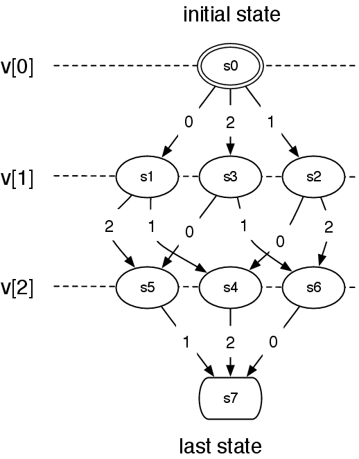
Each state can be assigned a level by topologically sorting states of the automaton. The variables from the list (second parameters) are assigned to these levels. All states at the same level are assigned the same variable (see Figure 3.2). If necessary, the automaton, containing cycles, is unrolled to match a list of variables. Each transitions has assigned values that are allowed for a variable when the transition in the automaton is selected. This is specified as the interval domain.
The example below implements the automaton from Figure 3.2. This automaton defines condition for three variables to be different values 0, 1 or 2.
   IntVar[] var = new IntVar[3];

   var[0] = new IntVar(store, "v"+0, 0, 2);

   var[1] = new IntVar(store, "v"+1, 0, 2);

   var[2] = new IntVar(store, "v"+2, 0, 2);


   FSM g = new FSM();

   FSMState[] s = new FSMState[8];

   for (int i=0; i<s.length; i++) {

      s[i] = new FSMState();

      g.allStates.add(s[i]);

   }

   g.initState = s[0];

   g.finalStates.add(s[7]);


   s[0].transitions.add(new FSMTransition(new IntervalDomain(0, 0),

                                          s[1]));

   s[0].transitions.add(new FSMTransition(new IntervalDomain(1, 1),

                                          s[2]));

   s[0].transitions.add(new FSMTransition(new IntervalDomain(2, 2),

                                          s[3]));


   s[1].transitions.add(new FSMTransition(new IntervalDomain(1, 1),

                                          s[4]));

   s[1].transitions.add(new FSMTransition(new IntervalDomain(2,2),

                                          s[5]));


   s[2].transitions.add(new FSMTransition(new IntervalDomain(0, 0),

                                          s[4]));

   s[2].transitions.add(new FSMTransition(new IntervalDomain(2,2),

                                          s[6]));


   s[3].transitions.add(new FSMTransition(new IntervalDomain(0, 0),

                                          s[5]));

   s[3].transitions.add(new FSMTransition(new IntervalDomain(1, 1),

                                          s[6]));


   s[4].transitions.add(new FSMTransition(new IntervalDomain(2, 2),

                                          s[7]));

   s[5].transitions.add(new FSMTransition(new IntervalDomain(1, 1),

                                          s[7]));

   s[6].transitions.add(new FSMTransition(new IntervalDomain(0, 0),

                                          s[7]));


   store.impose(new Regular(g, var));
Knapsack constraint specifies knapsack problem. This implementation2 was inspired by the paper [12] and published in [17]. The major extensions of that paper are the following. The quantity variables do not have to be binary. The profit and capacity of the knapsacks do not have to be integers. In both cases, the constraint accepts any finite domain variable.
The constraint specify number of categories of items. Each item has a given weight and profit. Both weight and profit are specified as positive integers. The problem is to select a number of items in each category to satisfy capacity constraint, i.e. the total weight must be in the limits specified by the capacity variable. Each such solution is then characterized by a given profit. It is defined in JaCoP as follows.
Knapsack(int[] profits, int[] weights, IntVar[] quantity,

         IntVar knapsackCapacity, IntVar knapsackProfit)
It can be formalize using the following constraints.
![∑
weights[i]⋅quantity[i] = knapsackCapacity
∑ i
profits[i]⋅quantity[i] = knapsackP rofit
i
∀i : weights[i] ∈ ℤ >0 ∧ ∀i : profits[i] ∈ ℤ >0](guideJaCoP6x.png) | (3.3) (3.4) (3.5) |
Geost is a geometrical constraint, which means that it applies to geometrical objects. It models placement problems under geometrical constraints, such as non overlapping constraints. Geost consistency algorithm was proposed by Beldiceanu et al [21]. The implementation of Geost in JaCoP is a result of a master thesis by Marc-Olivier Fleury.
In order to describe the constraint, we will introduce several definitions and relate them to JaCoP implementation.
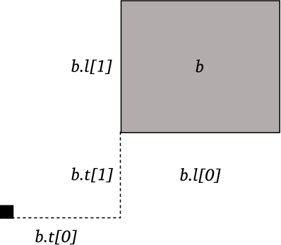
Definition 1 A shifted box b is a pair (b.t[],b.l[]) of vectors of integers of length k, where k is the number of dimensions of the problem. The origin of the box relative to a given reference is b.t[], and b.l[] contains the length of the box, for each dimension.
Shifted box is defined in JaCoP using class DBox. For example, a two dimensional shifted box starting at coordinates (0,0) and having length 2 in first dimension and 1 in second direction is specified as follows.
DBox sbox = new DBox(new int[] {0,0}, new int[] {2,1});
Definition 2 A shape s is a set of shifted boxes. It has a unique identifier s.sid.
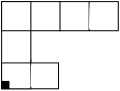
In JaCoP, we can define n shapes as collection of shifted boxes. Shape identifiers start at 0 and must be assigned consecutive integers. Therefore we have shapes with identifiers in interval 0..n-1. The following JaCoP example defines a shape with identifier 0, consisting of three sboxs, depicted in Figure 3.4.
    ArrayList<Shape> shapes = new ArrayList<Shape>();


    ArrayList<DBox> shape1 = new ArrayList<DBox>();

    shape1.add(new DBox(new int[] {0,0}, new int[] {2,1}));

    shape1.add(new DBox(new int[] {0,1}, new int[] {1,2}));

    shape1.add(new DBox(new int[] {1,2}, new int[] {3,1}));


    shapes.add( new Shape(0, shape1) );
Definition 3 An object o is a tuple (o.id,o.sid,o.x[], o.start,o.duration,o.end). o.id is a unique identifier, o.sid is a variable that stores all shapes that o can take. o.x[] is a k-dimensional vector of variables which represent the origin of o. o.start, o.duration and o.end define the interval of time in which o is present.
An object in JaCoP is defined by class GeostObject. It specifies basically all parameters of an object. An example below specifies object 0 that can take shapes 0, 1, 2 and 3. The object can be placed using coordinates (X_o1, Y_o1). The object is present during time 2 to 14.
    ArrayList<GeostObject> objects = new ArrayList<GeostObject>();


    IntVar X_o1 = new IntVar(store, "x1", 0, 5);

    IntVar Y_o1 = new IntVar(store, "y1", 0, 5);

    IntVar[] coords_o1 = {X_o1, Y_o1};

    IntVar shape_o1 = new IntVar(store, "shape_o1", 0, 3);

    IntVar start_o1 = new IntVar(store, "start_o1", 2, 2);

    IntVar duration_o1 = new IntVar(store, "duration_o1", 12, 12);

    IntVar end_o1 = new IntVar(store, "end_o1", 14, 14);

    GeostObject o1 = new GeostObject(0, coords_o1, shape_o1,

                                     start_o1, duration_o1, end_o1);

    objects.add(o1);
Note that since object shapes are defined in terms of collections of shifted boxes, and since shifted boxes have a fixed size, Geost is not suited to solve problems in which object sizes can vary. Polymorphism provides some flexibility (shape variable having multiple values in their domain), but it is essentially intended to allow the modeling of objects that can take a small amount of different shapes. Typically objects that can be rotated. The duration of an object can be useful in cases where objects have variable sizes, because it is a variable, which means that some more flexibility is available. However, this feature is only available for one dimension. These restrictions are design choices made by the authors of Geost, probably because it fits well their primary field of application, which consists in packing goods in trucks. Using fixed sized shapes is also useful because it allows more deductions concerning possible placements.
When all shapes and objects are defined it is possible to specify geometrical constraints that must be fulfilled when placing these objects. Implemented geometrical constraints include in-area and non-overlapping constraints. In-area constraint enforces that objects have to lie inside a given k-dimensional sbox. Non-overlapping constraints require that no two objects can overlap.
The code below specifies two geometrical constraint, non-overlapping and in-area. They are specified by classes NonOverlapping and InArea. It must be noted that non-overlapping constraint in the code below specifies that all objects must not overlap in its two dimensions and time dimension (the time dimension is implemented as one additional dimension and therefore we specify dimensions 0, 1 and 2). In-area constraint requires that all object must be included in the sbox of dimensions 5x4.
    ArrayList<ExternalConstraint> constraints =

                    new ArrayList<ExternalConstraint>();

    int[] dimensions = {0, 1, 2};

    NonOverlapping constraint1 =

                    new NonOverlapping(objects, dimensions);

    constraints.add(constraint1);

    InArea constraint2 = new InArea(

                  new DBox(new int[] {0,0}, new int[] {5,4}), null);

    constraints.add(constraint2);
Finally, the Geost constraint is imposed using the following code.
store.impose( new Geost(objects, constraints, shapes) );
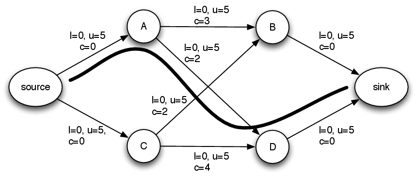
NetworkFlow constraint defines a minimum-cost network flow problem. An instance of this problem is defined on a directed graph by a tuple (N,A,l,u,c,b), where
N is the set of nodes,
A is the set of directed arcs,
l : A → ℤ≥0 is the lower capacity function on the arcs,
u : A → ℤ≥0 is the upper capacity function on the arcs,
c : A → ℤ is the flow cost-per-unit function on the arcs,
b : N → ℤ is the node mass balance function on the nodes.
A flow is a function x : A → ℤ≥0. The minimum-cost flow problem asks to find a flow that satisfies all arc capacity and node balance conditions, while minimizing total cost. It can be stated as follows:
| min | z(x) = ∑ (i,j)∈Acijxij | (3.6) |
| s.t. | lij ≤ xij ≤ uij ∀(i,j) ∈ A, | (3.7) |
| ∑ j:(i,j)∈Axij -∑ j:(j,i)∈Axji = bi ∀i ∈ N | (3.8) |
The network is built with NetworkBuilder class using node, defined by class org.jacop.net.Node and arcs. Each node is defined by its name and node mass balance b. For example, node A with balance 0 is defined using network net as follows.
    NetworkBuilder net = new NetworkBuilder();

    Node A = net.addNode("A", 0);
Source node producing flow of capacity 5 and sink node consuming flow of capacity 5 are defined using similar constructs but different value of node mass balance, as indicated below.
      Node source = net.addNode("source", 5);

      Node sink = net.addNode("sink", -5);
Arc of the network are defined always between two nodes. They define connection between given nodes, the lower and upper capacity values assigned to the arc (values l and u) as well as the flow cost-per-unit function on the arc (value c). This can be defined using different methods with either integers or finite domain variables. For example, an arc from source to node A with l = 0 and u = 5 and c = 3 can be defined as follows.
net.addArc(A, B, 3, 0, 5);
or
      x = new IntVar(store, "source->A", 0, 5);

      net.addArc(A, B, 3, x);
It can be noted, that cost-per-unit value can also be defined as a finite domain variable.
The constraint has also the flow cost, defined as z(x) in 3.6. It is defined as follows.
     IntVar cost = new IntVar(store, "cost", 0, 1000);

     net.setCostVariable(cost);
Note that the NetworkFlow only ensures that cost z(x) ≤ Zmax, where z(x) is the total cost of the flow (see equation (3.6)). In our code it is defined as variable cost.
The constraint is finally posed using the following method.
store.impose(new NetworkFlow(net));
For example, Figure 3.5 presents the code for network flow problem depicted in Figure 3.6. The minimal flow, found by the solver, is 10 that is indicated in the figure.
      store = new Store();


      IntVar[] x = new IntVar[8];


      NetworkBuilder net = new NetworkBuilder();

      Node source = net.addNode("source", 5);

      Node sink = net.addNode("sink", -5);


      Node A = net.addNode("A", 0);

      Node B = net.addNode("B", 0);

      Node C = net.addNode("C", 0);

      Node D = net.addNode("D", 0);


      x[0] = new IntVar(store, "x_0", 0, 5);

      x[1] = new IntVar(store, "x_1", 0, 5);

      net.addArc(source, A, 0, x[0]);

      net.addArc(source, C, 0, x[1]);


      x[2] = new IntVar(store, "a->b", 0, 5);

      x[3] = new IntVar(store, "a->d", 0, 5);

      x[4] = new IntVar(store, "c->b", 0, 5);

      x[5] = new IntVar(store, "c->d", 0, 5);

      net.addArc(A, B, 3, x[2]);

      net.addArc(A, D, 2, x[3]);

      net.addArc(C, B, 5, x[4]);

      net.addArc(C, D, 6, x[5]);


      x[6] = new IntVar(store, "x_6", 0, 5);

      x[7] = new IntVar(store, "x_7", 0, 5);

      net.addArc(B, sink, 0, x[6]);

      net.addArc(D, sink, 0, x[7]);


      IntVar cost = new IntVar(store, "cost", 0, 1000);

      net.setCostVariable(cost);


      store.impose(new NetworkFlow(net));
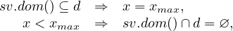
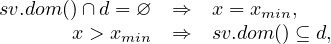
Network builder has a special attribute handlerList that makes it possible to specify structural rules connected to the network. Each structural rule must implement VarHandler interface, which allows network flow constraint to cooperate with the structural rule. An important, already implemented rule, is available in the class DomainStructure. It specifies, for each structural variable sv, a list of arcs that the structural rule influence. This structural rule makes it possible to enforce minimum or maximum amount of flow on a given arc depending on the relationship between the domain of variable sv and domain d, specified within a structural rule. The domain of variable sv and domain d do not intersect if and only if the flow on a given arc is minimal as specified by initial value x.min(), denoted as xmin. Moreover, the domain of varibale sv is contained within domain d if and only if the actual flow on a given arc is maximal as specified by initial value x.max(), denoted as xmax. It is enforced by the following rules.
 | (3.9) |
 | (3.10) |
For example, creation of structural rule for arc between node source and B will enforce that this arc will have maximal flow if variable s is zero and minimal flow otherwise. The rule works also in the other direction, i.e. if the flow will be maximal variable s=0 and if the flow will be minimal this variable will be 1.
      Arc[] arcs = new Arc[1];

      arcs[0] = net.addArc(source, B, 0, x[1]);


      IntVar s = new IntVar(store, "s", 0, 1);

      Domain[] domCond = new IntDomain[1];

      domCond[0] = new IntervalDomain(0, 0);


      net.handlerList.add(new DomainStructure(s,

                          Arrays.asList(domCond),

                          Arrays.asList(arcs)));
SoftAlldifferent constraint as well as SoftGCC constraint use DomainStructure rules to enforce flow from variable nodes to value nodes according the actual domain/value of variables represented by variable nodes. It is crucial functionality for the implementation of those soft global constraints.
Binpacking constraint defines a problem of packing bins with the specified items of a given size. Each bin has a defined load. The constraint is defined as follows.
Binpacking(IntVar[] item, IntVar[] load, int[] size)
where item means the bin number assigned to item at position i, load defines load of bin i as finite domain variable (min and max load) and size defines items i size.
It can be formalize using the following formulation.
![∑
∀i size[j] = load[i]
j whereitem[j]=i](guideJaCoP9x.png) | (3.11) |
The binpacking constraint implements methods and algorithms proposed in [24].
The LexOrder constraint enforces ascending lexicographic order between two vectors that can be of different size. The constraints makes it possible to enforce strict ascending lexicographic order, that is the fist vector must be always before the second one in the lexicographical order, or it can allow equality between the vectors. This is controlled by the last parameter of the constraint that is either true for strictly ascending lexicographic order or false otherwise. The default is non-strictly ascending lexicographic order when no second parameter is defined.
The following code specifies Lex constraint that holds when the strict ascending lexicographic order holds between two vectors of 0/1 varables.
      int N = 2;

      IntVar[] x = new IntVar[N];

      for (int i = 0; i < x.length; i++)

          x[i] = new IntVar(store, "x["+i+"]", 0, 1);


      IntVar[] y = new IntVar[N];

      for (int i = 0; i < y.length; i++)

          y[i] = new IntVar(store, "y["+i+"]", 0, 1);


      store.impose(new LexOrder(x, y, true));
The result is as follows.
[0, 0, 0], [0, 0, 1]

[0, 0, 0], [0, 1, 0]

[0, 0, 0], [0, 1, 1]

[0, 0, 0], [1, 0, 0]

[0, 0, 0], [1, 0, 1]

[0, 0, 0], [1, 1, 0]

[0, 0, 0], [1, 1, 1]

[0, 0, 1], [0, 1, 0]

[0, 0, 1], [0, 1, 1]

[0, 0, 1], [1, 0, 0]

[0, 0, 1], [1, 0, 1]

[0, 0, 1], [1, 1, 0]

[0, 0, 1], [1, 1, 1]

[0, 1, 0], [0, 1, 1]

[0, 1, 0], [1, 0, 0]

[0, 1, 0], [1, 0, 1]

[0, 1, 0], [1, 1, 0]

[0, 1, 0], [1, 1, 1]

[0, 1, 1], [1, 0, 0]

[0, 1, 1], [1, 0, 1]

[0, 1, 1], [1, 1, 0]

[0, 1, 1], [1, 1, 1]

[1, 0, 0], [1, 0, 1]

[1, 0, 0], [1, 1, 0]

[1, 0, 0], [1, 1, 1]

[1, 0, 1], [1, 1, 0]

[1, 0, 1], [1, 1, 1]

[1, 1, 0], [1, 1, 1]
The algorithm of this constraint is based on the algorithm presented in [8].
It defines value precedence constraint for integers. Value precedence is defined for integer value s, integer value t and an integer sequence x = [x0,...,xn-1] and means the following. If there exists j such that xj = t, then there must exist i < j such that xi = s. The algorithm is based on paper [14].
For example, the following code defines that 1 has to always proceed 4 in the sequence of four variables x (ValuePrecede) and, in addition x[2] = 4 (constraint XeqC).
    int N = 4;


    IntVar[] x = new IntVar[N];

    for (int i = 0; i < N; i++) {

        x[i] = new IntVar(store, "x["+i+"]", 1, N);

    }

    store.impose(new XeqC(x[2], 4));


    store.impose(new ValuePrecede(1, 4, x));
The resulting 24 solutions is as follows.
[x[0]=1, x[1]=1, x[2]=4, x[3]=1]

[x[0]=1, x[1]=1, x[2]=4, x[3]=2]

[x[0]=1, x[1]=1, x[2]=4, x[3]=3]

[x[0]=1, x[1]=1, x[2]=4, x[3]=4]

[x[0]=1, x[1]=2, x[2]=4, x[3]=1]

[x[0]=1, x[1]=2, x[2]=4, x[3]=2]

[x[0]=1, x[1]=2, x[2]=4, x[3]=3]

[x[0]=1, x[1]=2, x[2]=4, x[3]=4]

[x[0]=1, x[1]=3, x[2]=4, x[3]=1]

[x[0]=1, x[1]=3, x[2]=4, x[3]=2]

[x[0]=1, x[1]=3, x[2]=4, x[3]=3]

[x[0]=1, x[1]=3, x[2]=4, x[3]=4]

[x[0]=1, x[1]=4, x[2]=4, x[3]=1]

[x[0]=1, x[1]=4, x[2]=4, x[3]=2]

[x[0]=1, x[1]=4, x[2]=4, x[3]=3]

[x[0]=1, x[1]=4, x[2]=4, x[3]=4]

[x[0]=2, x[1]=1, x[2]=4, x[3]=1]

[x[0]=2, x[1]=1, x[2]=4, x[3]=2]

[x[0]=2, x[1]=1, x[2]=4, x[3]=3]

[x[0]=2, x[1]=1, x[2]=4, x[3]=4]

[x[0]=3, x[1]=1, x[2]=4, x[3]=1]

[x[0]=3, x[1]=1, x[2]=4, x[3]=2]

[x[0]=3, x[1]=1, x[2]=4, x[3]=3]

[x[0]=3, x[1]=1, x[2]=4, x[3]=4]
Member constraint enforces that an element e is present on a list x and is defined as follows.
Member(IntVar[] x, IntVar e)
where x is a list of variables and e is the element. The constraint is primitive and can be used in different context as a parameter of other constraints.
Channeling constraints are generalizations of simple Reified and Implies constraints.
ChannelReif enforces the following constrains in one global constraint.
∀i x=i<=>bi
The above constraints are specified using a single ChannelReif constraint.
ChannelReif(x, b);
where x is a IntVar and b is vector of 0..1 variables.
Similarly, ChannelImply enforces the following constrains in one global constraint.
∀i bi=>x=i
More advanced versions of these constraints make it possible to specify possible values checked for variable x. For more details check API documentation.
Decomposed constraints do not define any new constraints and related pruning algorithms. They are translated into existing JaCoP constraints. Sequence and Stretch constraints are decomposed using Regular constraint.
Decomposed constraints are imposed using imposeDecomposition method instead of ordinary impose method.
Sequence constraint restricts values assigned to variables from a list of variables in such a way that any sub-sequence of length q contains N values from a specified set of values. Value N is further restricted by specifying min and max allowed values. Value q, min and max must be integer.
The following code defines restrictions for a list of five variables. Each sub-sequence of size 3 must contain 2 (min = 2 and max = 2) values 1.
   IntVar[] var = new IntVar[5];

   for (int i=0; i<var.length; i++)

      var[i] = new IntVar(store, "v"+i, 0, 2);


   store.imposeDecomposition(new Sequence(var, //variable list

                        new IntervalDomain(1,1), //set of values

                        3, // q, sequence length

                        2, // min

                        2  // max

                      ));
There exist ten solutions: [01101, 01121, 10110, 10112, 11011, 11211, 12110, 12112, 21101, 21121]
Stretch constraint defines what values can be taken by variables from a list and how sub-sequences of these values are formed. For each possible value it specifies a minimum (min) and maximum (max) length of the sub-sequence of these values.
For example, consider a list of five variables that can be assigned values 1 or 2. Moreover we constraint that the sub-sequence of value 1 must have length 1 or 2 and the sub-sequence of value 2 must have length either 2 or 3. The following code specifies these restrictions.
   IntVar[] var = new IntVar[5];

   for (int i=0; i<var.length; i++)

      var[i] = new IntVar(store, "v"+i, 1, 2);


   store.imposeDecomposition(

                     new Stretch(new int[] {1, 2},  // values

                                 new int[] {1, 2},  // min for 1 & 2

                                 new int[] {2, 3},  // max for 1 & 2

                                 var // variables

                            ));
This program produces six solutions: [11221, 11222, 12211, 12221, 22122, 22211]
The Lex constraint enforces ascending lexicographic order between n vectors that can be of different size. The constraints makes it possible to enforce strict ascending lexicographic order, that is vector i must be always before vector i + 1 in the lexicographical order, or it can allow equality between consecutive vectors. This is controlled by the last parameter of the constraint that is either true for strictly ascending lexicographic order or false otherwise. The default is non-strictly ascending lexicographic order when no second parameter is defined.
The following code specifies Lex constraint that holds when the strict ascending lexicographic order holds between four vectors of different sizes.
      IntVar[] d = new IntVar[6];

      for (int i = 0; i < d.length; i++) {

          d[i] = new IntVar(store, "d["+i+"]", 0, 2);

      }


      IntVar[][] x = { {d[0],d[1]}, {d[2]}, {d[3],d[4]}, {d[5]} };


      store.imposeDecomposition(new Lex(x, true));
This program produces nine following solutions.
[[0, 0], [1], [1, 0], [2]],
[[0, 0], [1], [1, 1], [2]],
[[0, 0], [1], [1, 2], [2]],
[[0, 1], [1], [1, 0], [2]],
[[0, 1], [1], [1, 1], [2]],
[[0, 1], [1], [1, 2], [2]],
[[0, 2], [1], [1, 0], [2]],
[[0, 2], [1], [1, 1], [2]],
[[0, 2], [1], [1, 2], [2]]
Soft-alldifferent makes it possible to violate to some degree the alldifferent relation. The violations will come at a cost which is represented by cost variable. This constraint is decomposed with the help of network flow constraint.
There are two violation measures supported, decomposition based, where violation of any inequality relation between any pair contributes one unit of cost to the cost metric. The other violation measure is called variable based, which simply states how many times a variable takes value that is already taken by another variable.
The code below imposes a soft-alldifferent constraint over five variables with cost defined as being between 0 and 20.
   IntVar[] x = new IntVar[5];

   for (int i=0; i< x.length; i++)

      x[i] = new IntVar(store, "x"+i, 1, 4);

   IntVar cost = new IntVar(store, "cost", 0, 20);


   store.imposeDecomposition(new SoftAlldifferent(x, cost,

                             ViolationMeasure.DECOMPOSITION_BASED );
Soft-GCC constraint makes it possible to violate to some degree GCC constraint. The Soft-GCC constraint requires number of arguments. In the code example below, vars specify the list of variables, which values are being counted, and the list of integers countedValues specifies the values that are counted. Values are counted in two counters specified by a programmer. The first list of counter variables, denoted by hardCounters in our example, specifies the hard limits that can not be violated. The second list, softCounters, specifies preferred values for counters and can be violated. Each position of a variable on these lists corresponds to the position of the value being counted on list countedValues. In practice, domains of variables on list hardCounters should be larger than domains of corresponding variables on list softCounters.
Soft-GCC accepts only value based violation metric that, for each counted value, sums up the shortage or the excess of a given value among vars. There are other constructors of Soft-GCC constraint that allows to specify hard and soft counting constraints in multitude of different ways.
store.imposeDecomposition(new SoftGCC(vars, hardCounters,

                          countedValues, softCounters,

                          cost, ViolationMeasure.VALUE_BASED));
JaCoP provides a library of set constraints in library org.jacop.set. This implementation is based on set intervals and related operations as originally presented in [9] and the first version has been implemented as a diploma project1 . JaCoP definition of set intervals, set domains and set variables is presented in section 4.1. Available constraints are discussed in section 4.2. Search, using set variables, is introduced in section 4.3.
Set is defined as an ordered collection of integers using class org.jacop.core.IntervalDomain and a set domain as abstract class org.jacop.set.core.SetDomain. Currently, there exist only one implementation of set domain as a set interval, called BoundSetDomain. The set interval for BoundSetDomain d is defined by its greatest lower bound (glb(d)) and its least upper bound (lub(d)). For example, set domain d = {{1}..{1..3}} is defined with glb(d) = {1}, set containing element 1, and lub(d) = {1..3}, set containing elements 1, 2 and 3. This set domain represent a set of sets {{1},{1..2},{1,3},{1..3}}. Each set domain to be correct must have glb(d) ⊆ lub(d). glb(d) can be considered as a set of all elements that are members of the set and lub(d) specifies the largest possible set.
The following statement defines set variable s for the set domain discussed above.
SetVar s = new SetVar(store, "s",

      new BoundSetDomain(new IntervalDomain(1,1),

                         new IntervalDomain(1,3)));
BoundSetDomain can specify a typical set domain, such as d = {{}..{1..3}}, in a simple way as
SetVar s = new SetVar(store, "s", 1, 3);
and an empty set domain as
SetVar s = new SetVar(store, "s", new BoundSetDomain());
Set domain can be created using IntervalDomain and BoundSetDomain class methods. They make it possible to form different sets by adding elements to sets.
JaCoP implements a number of set constraints specified in appendix A.2. Constraints AinS, AeqB and AinB are primitive constraints and can be reified and used in other constraints, such as conditional and logical. Other constraints are treated as ordinary JaCoP constraints.
Consider the following code that uses union constraint.
SetVar s1 = new SetVar(store, "s1",

                new BoundSetDomain(new IntervalDomain(1,1),

                                   new IntervalDomain(1,4)));

SetVar s2 = new SetVar(store, "s2",

                new BoundSetDomain(new IntervalDomain(2,2),

                                   new IntervalDomain(2,5)));

SetVar s = new SetVar(store, "s", 1,10);

Constraint c = new AunionBeqC(s1, s2, s);
It performs operation {{1}..{1..4}} ⋃ {{2}..{2..5}} = {{}..{1..10}} and produces {{1}..{1..4}} ⋃ {{2}..{2..5}} = {{1..2}..{1..5}}. This represents 108 possible solutions.
Set variables will require different search organization. Basically, during search the decisions will be made whether an element belongs to a set or it does not belong to this set.
JaCoP still uses DepthFirstSearch but needs different methods for set variable selection implementing ComparatorVariable and a method for value selection implementing Indomain. The special methods are specified in appendix B.2. In addition, variable selection methods MostConstrainedStatic and MostConstrainedDynamic will also work.
An example search can be specified as follows.
   Search<SetVar> search = new DepthFirstSearch<SetVar>();


   SelectChoicePoint<SetVar> select = new SimpleSelect<SetVar>(

                                vars,

                                new MinLubCard<SetVar>(),

                                new MaxGlbCard<SetVar>(),

                                new IndomainsetMin<SetVar>());

   search.setSolutionListener(new SimpleSolutionListener<SetVar>());


   boolean result = search.labeling(store, select);
JaCoP provides a library of floating point constraints in library org.jacop.floats. This implementation is based on floating point intervals and related constraints.
Floating point domain is defined in a similar way as integer variable domain as an ordered list of floating point intervals in class org.jacop.floats.core.FloatIntervalDomain. This class implements an abstract class org.jacop.floats.core.FloatDomain that in turn extends ordinary JaCoP domain defined in org.jacop.core.Domain. The floating point variable is defined using the floating point interval as follows.
FloatVar f = new FloatVar(store, "f", 0.0, 10.0);
This java declaration defines floating point variable f with domain 0.0..10.0.
The float variables are used in floating point constraints, discussed in the next section. Special attention is paid to precision of floating point operations. Basically, JaCoP considers a floating point interval to represent a single value if a difference between max and min values of a variable is lower than an epsilon value (ϵ). Epsilon is calculated based on a given precision and ulp value (ulp is a floating point specific value know as “unit at last position”). The precision is defined in org.jacop.core.FloatDomain and can be set-up and obtained using following methods FloatDomain.setPrecision(double p) and FloatDomain.precision(). Epsilon is defined as a maximum of ulp and the precision. Class FloatDomain defines also min and max values of floating variables and values of π and e.
JaCoP implements a number of floating point constraints specified in appendix A.3.
Constraints PeqC, PeqQ, PgtC, PgtQ, PgteqC, PgteqQ, PltC, PltQ, PlteqC, PlteqQ, PneqC, PneqQ, PplusCeqR,PplusQeqR, PminusCeqR, PminusQeqR and LinearFloat are primitive constraints and can be reified and used in other constraints, such conditional and logical. Other constraints are treated as ordinary JaCoP constraints.
Consider the following code that uses division constraint.
FloatDomain.setPrecision(1E-4);


FloatVar a = new FloatVar(store, "a", 0.1, 3.0);

FloatVar b = new FloatVar(store, "b", -0.2, 6.0);

FloatVar c = new FloatVar(store, "c", -1000, 1000);


store.impose(new PdivQeqR(a, b, c));
It performs operation {0.100..3.000} / {-0.200..6.000} and produces a pruned domain for c::{-1000.0000..-0.5000, 0.0167..1000.0000}, assuming precision 10-4.
Floating point variables will require special search definition. Basically, a domain split search (bisection) is used together with consistency checking to find a solution.
JaCoP standard search for floating point variables still uses DepthFirstSearch but needs to use specific methods for selection of choice points as well as variable selection. org.jacop.floats.search.SplitSelectFloat is used to define how intervals of floating point variables will be split. Default behavior of this method is to split an interval in a middle and try the left part first. If variable leftFirst is set to false the right interval will be checked first. The variables will be selected based on the variable selection heuristic defined as a parameter for SplitSelectFloat class. There exist several methods to select variables specific for FloatVar. They are defined in org.jacop.floats.search. Other general methods that are not specific for a given domain can also be used here, for example org.jacop.search.MostConstrainedStatic.
An example search can be specified as follows.
DepthFirstSearch<FloatVar> search = new DepthFirstSearch<FloatVar>();

SplitSelectFloat<FloatVar> select = new SplitSelectFloat<FloatVar>(

                               store, x,

                               new LargestDomainFloat<FloatVar>());

search.setSolutionListener(new PrintOutListener<FloatVar>());


boolean result = search.labeling(store, select);
Minimization, using DepthFirstSearch class, is done as for other variables by calling labeling method with the third parameter defining cost variable. Both IntVar and FloatVar can be used to defined cost criteria for minimization.
JaCoP offers also another minimization method. This method uses cost variable to lead the minimization. The method splits the domain of cost variable into two parts and then checks, using standard DepthFirstSearch labeling method if there is a solution in this part. If there is a solution in this part it continues to split the current interval and checks the left interval again. If there is no solution in this part (depth-first-search return false) it will try the right interval. The search finishes when the cost variable is ground (the difference between max and min is lower or equal epsilon). An example code is presented below.
DepthFirstSearch<FloatVar> search = new DepthFirstSearch<FloatVar>();

SplitSelectFloat<FloatVar> select = new SplitSelectFloat<FloatVar>(

                           store, x,

                           new LargestDomainFloat<FloatVar>());


Optimize min = new Optimize(store, search, select, cost);

boolean result = min.minimize();
It is also possible to define SplitSelectFloat with variable selection heuristic (the last parameter) equal null. In this case a default method will be used that is round-robin selection. The variables are selected in a round-robin fashion until their domains will not become ground.
The following code defines equation x2 + sin(1∕x3) = 0 together with the search that finds all 318 solutions.
FloatDomain.setPrecision(1.0e-14);

FloatDomain.intervalPrint(false);

Store store = new Store();


FloatVar x = new FloatVar(store, "x", 0.1, 1.0);

FloatVar zero = new FloatVar(store, 0,0);

FloatVar one = new FloatVar(store, 1,1);


// x*x + sin(1.0/(x*x*x)) = 0.0;

FloatVar[] temp = new FloatVar[4];

for (int i=0; i<temp.length; i++)

    temp[i] = new FloatVar(store, "temp["+i+"]", -1e150, 1e150);

store.impose(new PmulQeqR(x, x, temp[0]));

store.impose(new PmulQeqR(x, temp[0], temp[1]));

store.impose(new PdivQeqR(one, temp[1], temp[2]));

store.impose(new SinPeqR(temp[2], temp[3]));

store.impose(new PplusQeqR(temp[0], temp[3], zero));


DepthFirstSearch<FloatVar> search = new DepthFirstSearch<FloatVar>();

SplitSelectFloat<FloatVar> s = new SplitSelectFloat<FloatVar>(store,

                                   new FloatVar[] {x}, null);

search.setSolutionListener(new PrintOutListener<FloatVar>());

search.getSolutionListener().searchAll(true);


search.labeling(store, s);
The last solution is x = 0.65351684593772.
JaCoP package org.jacop.floats offers also experimental extensions. They include a method to generate constraints that define the derivative of a function, represented by constraints, and a interval Newton method.
JaCoP can do symbolic (partial) derivatives of functions, that is using the defined constraints for a given function and a variable defining the result of the function, JaCoP will generate constraints that define a function for a derivative of the original function. There is a complication in this process since constraints are not functions and sometime it is difficult or impossible to find out which constraint defines a function for a given variable. In such situations JaCoP uses a heuristic to find out this but it is also possible to define this explicitly. The following examples explains the process of computing derivatives of constrains.
Set<FloatVar> vars = new HashSet<FloatVar>();

vars.add(x1);

vars.add(x2);

Derivative.init(store);

// Derivative.defineConstraint(x1x1, c0);

// Derivative.defineConstraint(x2x2, c1);

// Derivative.defineConstraint(x1x1x1x1, c2);

// Derivative.defineConstraint(x2x2x2x2, c3);


// ================== df/dx1 =================

FloatVar fx1 = Derivative.getDerivative(store, f, vars, x1);


// ================== df/dx2 =================

FloatVar fx2 = Derivative.getDerivative(store, f, vars, x2);
In the above example, JaCoP will generate two partial derivatives  and
and  . Set vars
is used to keep all variables of function defined by variable f. The function defined by
variable f is usually defined by several constraints using temporary variables, such as x1x1,
x2x2, x1x1x1x1 and x2x2x2x2. In such situations JaCoP tries, using heuristics, to find out
what constraint defines a given temporary variable. Sometimes it is not possible and the
programmer needs to define it, as indicated by the commented code and methods
Derivative.defineConstraint. For example, constraint c0 defines variable x1x1. Method
getDerivative of class Derivative generates a variable that defines the result of the
derivative.
. Set vars
is used to keep all variables of function defined by variable f. The function defined by
variable f is usually defined by several constraints using temporary variables, such as x1x1,
x2x2, x1x1x1x1 and x2x2x2x2. In such situations JaCoP tries, using heuristics, to find out
what constraint defines a given temporary variable. Sometimes it is not possible and the
programmer needs to define it, as indicated by the commented code and methods
Derivative.defineConstraint. For example, constraint c0 defines variable x1x1. Method
getDerivative of class Derivative generates a variable that defines the result of the
derivative.
Derivatives, can be used for setting additional constraints on solutions. For example, when looking for minimum or maximum of a function or in the interval Newton method.
Interval Newton methods combine classical Newton method with interval analysis [13] and are used to provide better bounds on variables.
Traditionally, univariate Newton method computes a solution for equation f(x) = 0 using the following approximation.
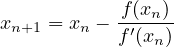 |
This can be extended by using vector x and a Jacobian matrix instead of f′(x). Furthermore one can extend it to interval arithmetic. This is implemented in JaCoP using “constraint” EquationSystem. This constraint takes as parameters a vector of functions and variables of these functions. The constraints computes then all partial derivatives and form a set of equations that are later solved, if possible, by interval Gauss-Seidel method.
This can be formalized as system of linear equations that, when solved, provides bounds on values (xn+1 - xn) of variables of equations.
 |
Below, constraint eqs specifies a set of two functions f0 and f1 of two variables x1 and x2. Constraint eqs will try to prune domains of variables x1 and x2.
EquationSystem eqs = new EquationSystem(store,

       new FloatVar[] {f0, f1}, new FloatVar[] {x1, x2});

store.impose(eqs);
JaCoP offers methods for finding a single solution, all solutions and a solution that minimizes a given cost function. These methods are used together with methods defining variable selection and assignment of a selected value to variable. Both complete search methods and heuristic search methods can be defined in JaCoP.
JaCoP offers powerful methods for search modification, called search plug-ins. Search plug-ins can be used both for collecting information about search as well as for changing search behaviour. For more information on search plug-ins see section 6.4.
A solution satisfying all constraints can be found using a depth first search algorithm. This algorithm searches for a possible solution by organizing the search space as a search tree. In every node of this tree a value is assigned to a domain variable and a decision whether the node will be extended or the search will be cut in this node is made. The search is cut if the assignment to the selected domain variable does not fulfill all constraints. Since assignment of a value to a variable triggers the constraint propagation and possible adjustment of the domain variable representing the cost function, the decision can easily be made to continue or to cut the search at this node of the search tree.
Typical search method for a single solution, for a list of variables, is specified as follows.
   Search<T> search = new DepthFirstSearch<T>();

   SelectChoicePoint<T> select = new SimpleSelect<T>(var,

                                               varSelect,

                                               tieBreakerVarSelect

                                               indomain);

   boolean result = search.labeling(store, select);
where T is type of variables we are using for this search (usually IntVar or SetVar), var is
a list of variables, varSelect is a comparator method for selecting variable and
tieBreakerV arSelect is a tie breaking comparator method. The tie breaking method is used
when the varSelect method cannot decide ordering of two variables. Finally, indomain
method is used to select a value that will be assigned to a selected variable. Different variable
selection and indomain methods are specified in appendix B. This search, for variables of
type IntVar creates choice points xi = val and xi≠val where xi is variable identified
by variable selection comparators and val is the value determined by indomain
method. For variables of type SetVar the choice is made between val ∈ xi or
val xi.
xi.
The standard method can be further modified to create search for all solutions. This is achieved by adopting the standard solution listener as specified below.
   search.getSolutionListener().searchAll(true);

   search.getSolutionListener().recordSolutions(true);
In the first line the flag that changes search to find all solutions is set. It is set in the default solution listener. In this example, we also set a flag that informs search to record all found solutions. If this flag is not set the search will only count solutions without storing them. The values for found solutions can be printed using label.getSolutionListener().printAllSolutions() method or the following piece of code.
   for (int i=1; i<=label.getSolutionListener().solutionsNo(); i++){

      System.out.print("Solution " + i + ": ");

      for (int j=0; j<label.getSolution(i).length; j++)

         System.out.print(label.getSolution(i)[j]);

      System.out.println();

   }
Even if the solutions are not recorded, they are counted and number of found solutions can be retrieved using method search.getSolutionListener().solutionsNo().
The minimization in JaCoP is achieved by defining variable for cost and using branch-and-bound (B&B) search, as specified below.
   IntVar cost;

   ...

   boolean result = search.labeling(store, select, cost);
B&B search uses depth-first-search to find a solution. Each time a solution with cost costV aluei is found a constraint cost < costV aluei is imposed. Therefore the search finds solutions with lower cost until it eventually fails to find any solution that proves that the last found solution is optimal, i.e., there is no better solution.
Sometimes we want to interrupt search and report the best solution found in a given time. For this purpose, the search time-out functionality can be used. For example, 10s time-out can be set with the following statement.
search.setTimeOut(10);
Moreover, one can define own time-out listener to perform specific actions.
In some situation classical depth first search algorithm is not best suited for finding a solution or finding an optimal solution. In such situation a so called restart search can be used. This search method runs an ordinary depth first search and then restarts the search from the beginning. Restarting of the search is forced when certain conditions are met. In our case, we restart search if a given number of fails occurred. Therefore, restart search takes as parameters, the specification of the depth first search, the calculator for providing a limit on fails and possibly a cost variable. An example code for defining restart search is as follows.
    import org.jacop.search.restart.*;


    DepthFirstSearch<IntVar> label = new DepthFirstSearch<>();

    SelectChoicePoint<IntVar> select = new SplitSelect<>(vars,

                        new ActivityMax<IntVar>(store),

                        new IndomainMin<IntVar>());


    RestartSearch<IntVar> rs = new RestartSearch<>(store, label,

                        select,

                        new LubyCalculator<IntVar>(2000),

                        cost);

    boolean result = rs.labeling();
Depth first search, label is defined as usually with select method that uses variable selection method ActivityMax, that is it will selects variables that are most often pruned. This makes possible to select variables in different order when restart happens. Restart search uses Luby calculator to give the number of allowed fails. It starts from 2000 fails and then uses a Luby number to multiply by 2000 on consecutive restarts to compute the limit on the number of fails. Other calculators are also available.
The restart search works also with the depth first search method defined as a sequence of several search methods.
It is a good strategy to add a solution listener to the last search or add default solution listener to restart search by calling RestartSearch method rs.addReporter(new CustomReport(vars)).
Finally, to make restart search effective one has to define it in such a way that it would use a different variable ordering and/or value assignment on different restarts. In the example above we have used ActivityMax variable selection heuristic that dynamically changes the order of selected variables based on their pruning statistics. The other similar methods are based on accumulated failure count (afc). Value selection can use, for example, random value assignment.
Priority search specifies complex nested searches [7]. A vector of variables is used to select a search that will be explored next. An example code below defines a priority search that based on variables p selects one of dfs[i] depth-first-searches to execute. All searches are connected and can be considered as one depth-first-search.
IntVar[] p = new IntVar[n];

p[0] = new IntVar(store, "p[0]", 2,2);

p[1] = new IntVar(store, "p[1]", 1,1);

p[2] = new IntVar(store, "p[2]", 3,3);


d = new IntVar[3][2];


IntVar[] vs = new IntVar[6];

int k=0;

for (int i = 0; i < n; i++)

  for (int j = 0; j < 2; j++) {

    d[i][j] = new IntVar(store, "d["+i+"]["+j+"]", 0, 5);

    vs[k++] = d[i][j];

  }

store.impose(new Alldiff(vs));


DepthFirstSearch[] search = new DepthFirstSearch[3];

for (int i = 0; i < n; i++) {

  DepthFirstSearch<IntVar> dfs = new DepthFirstSearch<>();

  dfs.setSelectChoicePoint(new InputOrderSelect<IntVar>(store,

                           d[i], new IndomainMin<IntVar>()));

  dfs.setPrintInfo(false);

  search[i] = dfs;

}


PrioritySearch<IntVar> label = new PrioritySearch<IntVar>(p,

                  new SmallestMin<IntVar>(), search);

label.setPrintInfo(false);

label.setSolutionListener(new Printer());

label.setAssignSolution(true);

label.getSolutionListener().recordSolutions(true);


cost = d[1][1];

boolean result = label.labeling(store,cost);


class Printer<T extends Var> extends SimpleSolutionListener<T> {


  public boolean executeAfterSolution(Search<T> search,

                                    SelectChoicePoint<T> select) {


    boolean returnCode = super.executeAfterSolution(search, select);


    System.out.println(cost);

    System.out.print("d = [ ");

    for (int i = 0; i < d.length; i++)

        System.out.print(java.util.Arrays.asList(d[i])+" ");

    System.out.println("]");

    System.out.println("---------");

    return returnCode;

  }

}
PrioritySearch extends DepthFirstSearch and takes as arguments a vector of variables used for search selection, variables selection method and a vector of searches. During search it selects a search from a vector of searches and executes it. Selection is controlled by selection variables and specified variable selection method. For the example above searches are selected in the following order dfs[1], dfs[0] and dfs[2]. The resulting solutions, printed by Printer are following.
d[1][1] = 1

d = [ [d[0][0] = 2, d[0][1] = 3] [d[1][0] = 0, d[1][1] = 1] [d[2][0] = 4, d[2][1] = 5] ]

---------

d[1][1] = 0

d = [ [d[0][0] = 2, d[0][1] = 3] [d[1][0] = 1, d[1][1] = 0] [d[2][0] = 4, d[2][1] = 5] ]

---------
PrioritySearch can be combined with other search combinators. It can be part of sequence of searches, each search in the vector of searches can also be a sequence of searches. Finally, restart search can use this search or combination of searches.
The search-plugin is an object, which is informed about the current state of the search and may influence the behavior of the search. They are divided into search-plugins that change the search behavior and plugins used for collecting and sharing information. Table 6.1 lists the search-plugins available in JaCoP and their membership in a respective group.
The search plug-ins are called during search when they reach a specific state, as specified below.
Solution listener plug-in is called by search when a solution is found
Exit child listener plug-in is called every time the search exits the search subtree (it has four different methods; two methods, which are called when the search has exited the left subtree and two methods for the right subtree).
Consistency listener plug-in is called after consistency method at the current search node.
Exit listener plug-in is called each time the search is about to exit (it can be used to collect relevant search information).
Time-out listener plug-in is called when the time-out occurs (if specified).
Initialize listener plug-in is called at the beginning of the search.
Changing search plug-ins can override the status of the search by returning true or false status. For example, exit child listener method leftChild can override the status of the search by returning true or false status. If it returns true then the search continues and enters the right child to keep looking for a solution. Returning false instructs the search to skip exploring the right subtree
JaCoP makes it possible to combine several plugins hierarchically. Each listener may have multiple children listeners attached to it, which have potential to influence the behaviour of the parent. A very simple example of using this behavior, is using one listener to remember solution and another one to print it. These two different functionalities may be provided by two different listeners. In general, if search calls several children listeners the parent listener decides how to treat the results returned by them. The listeners already implemented in JaCoP use the following default rule to combine the return codes from different listeners. They combine their own return code with the return code of a child listener using conjunction of return codes. Several child listeners combine their return codes using disjunction of return codes.
Credit search combines credit based exhaustive search at the beginning of the tree with local search in the rest of the tree [2]. In JaCoP, the credit search is controlled by three parameters: number of credits, number of backtracks during local search and maximum depth of search. In Figure 6.1 there is an example of the credit search tree. The search has initially 8 credits. The number of possible backtracks is three. During search half of the credits is distributed to the selected choice. The rest of the credits is distributed using the same principle for the next choice point. The first part of the search is based on the credits and makes it possible to investigate many possible assignments to domain variables while the other part is supposed to lead to a solution and can use a number of backtracks specified for this search. Moreover, the maximal depth of the search cannot be exceeded. Since we control the search it is possible to partially explore the whole tree and avoid situations when the search is stuck at one part of the tree which is a common problem of B&B algorithm when a depth first search strategy is used.
An example of the command which produces the search tree depicted in Fig. 6.1 is as follows.
   SelectChoicePoint<IntVar> select = new SimpleSelect<IntVar>(vars,

                                       new SmallestDomain<IntVar>(),

                                       new IndomainMin<IntVar>());


   int credits=8, backtracks=3, maxDepth=1000;

   CreditCalculator<IntVar> credit = new CreditCalculator<IntVar>(

                                                  credits,

                                                  backtracks,

                                                  maxDepth);

   Search<IntVar> search = new DepthFirstSearch<IntVar>();

   search.setConsistencyListener(credit);

   search.setExitChildListener(credit);

   search.setTimeOutListener(credit);


   boolean result = search.labeling(store, select);
Limited discrepancy search (LDS) uses the partial search method proposed in [11]. It basically allows only a number of different decisions along a search path, called discrepancies. If the number of discrepancies is exhausted backtracking is initiated. The number of discrepancies is specified as a parameter for LDS.
An example of LDS with one discrepancy is as follows.
   Search<IntVar> search = new DepthFirstSearch<IntVar>();

   SelectChoicePoint<IntVar> select = new SimpleSelect<IntVar>(var,

                                      new SmallestDomain<IntVar>(),

                                      new IndomainMiddle<IntVar>());

   LDS<IntVar> lds = new LDS<IntVar>(2);

   search.setExitChildListener(lds);


   boolean result = search.labeling(store, select);
JaCoP offers, through its plug-ins, possibility to combine several search methods into a single complex search. For example, the following code presents a search that is build as consecutive invocation of two search methods.
   Search<IntVar> slave = new DepthFirstSearch<IntVar>();

   SelectChoicePoint<IntVar> selectSlave =

          new SimpleSelect<IntVar>(vars2,

                                   new SmallestMin<IntVar>(),

                                   new SmallestDomain<IntVar>(),

                                   new IndomainMin<IntVar>());

   slave.setSelectChoicePoint(selectSlave);


   Search<IntVar> master = new DepthFirstSearch<IntVar>();

   SelectChoicePoint<IntVar> master =

          new SimpleSelect<IntVar>(vars1,

                                   new SmallestMin<IntVar>(),

                                   new SmallestDomain<IntVar>(),

                                   new IndomainMin<IntVar>());

   master.addChildSearch(slave);


   boolean result = master.labeling(store, selectMaster);
When several search methods is combined to form a sequential search and the minimization is done one has to set for each sub-search a flag informing this search that it is a part of minimization. It is achieved by the following instruction.
slave.setOptimize(true);
JaCoP has a SAT solver that can be used together with JaCoP solver. It has
been developed by Simon Cruanes and Radosław Szymanek. The SAT solver can
be integrated in JaCoP as a SAT constraint and used with JaCoP search methods.
This functionality is offered by a org.jacop.satwrapper.SatWrapper class.
Typical translation of Boolean constraints, used in flatzinc compilations are defined in
org.jacop.satwrapper.SatTranslation.
Typical Boolean formulas can be added to SAT solver using class SatTranslation. This class offers translation of typical operations as and, or, not, xor, implication, all equalities and inequalities as well as reified versions of these. The following code illustrates use of the translation.
   SatTranslation sat = new SatTranslation(store);

   sat.impose(); // impose SAT-solver as constraint


   BooleanVar a = new BooleanVar(store, "a");

   BooleanVar b = new BooleanVar(store, "b");

   BooleanVar c = new BooleanVar(store, "c");


   // adding SAT clauses

   sat.generate_implication(a, b);

   sat.generate_and(new BooleanVar[] {a, b}, c);
The code generates Boolean clause of the form (a → b) ∧ (a∧b = c) that is translated to CNF Boolean clause supported by the SAT solver.
(a ∨ b) ∧
(a ∨b ∨ c) ∧
(a ∨c) ∧
(b ∨c)
The SAT translation performs several tasks. First, it defines SAT literals and binds Boolean variables to these literals. In our example, Boolean variables a, b and c are translated to literals, denoted by the same letter in the above formulas but they are different representations. Second, it adds CNF clauses representing Boolean clauses to the SAT solver. The SAT wrapper will then propagate changes between CP and SAT solver based on the evaluations of both solvers.
The search for solutions is identical with CP framework. In case of the example, we can make search on variables a, b and c. All solutions to the constraint are {0, 0, 0}, {0, 1, 0}, {1, 1, 1}
SatWrapper offers a general way to define literals and clauses. The process is divided into two parts. First, each FDV and a inequality relation on it is bound to a literal. Then a clause is defined on the literals. We illustrate this process below.
Assume that we want to define a constraint (a ≤ 10) → (b = 3 ∧c > 7) with IntVar a, b and c. The literals for this constraint are defined as ⟦a ≤ 10⟧, ⟦b = 3⟧ and ⟦c ≤ 7⟧ (negation of this literal is a > 7). This is encoded in JaCoP as follows.
   IntVar a = new IntVar(store, "a", 0, 100);

   IntVar b = new IntVar(store, "b", 0, 100);

   IntVar c = new IntVar(store, "c", 0, 100);


   SatWrapper wrapper = new SatWrapper();

   store.impose(wrapper);


   wrapper.register(a);

   wrapper.register(b);

   wrapper.register(c);


   int aLiteral = wrapper.cpVarToBoolVar(a, 10, false);

   int bLiteral = wrapper.cpVarToBoolVar(b, 3, true);

   int cLiteral = wrapper.cpVarToBoolVar(c, 7, false);
In the above method cpVarToBoolVar the first parameter is the FDV variable, the second is the rhs value and the third parameter defines type if relation (false for ≤ and true for =).
When literals are defined we can generate clauses using CNF format, as presented below. First, we translate the clause to CNF form as (⟦a ≤ 10⟧∨⟦b = 3⟧) ∧ (⟦a ≤ 10⟧∨⟦c ≤ 7⟧). Then we encode this into JaCoP SAT solver.
   IntVec clause = new IntVec(wrapper.pool);


   // first clause

   clause.add(- aLiteral);

   clause.add(bLiteral);

   wrapper.addModelClause(clause.toArray());


   clause = new IntVec(wrapper.pool);


   // second clause

   clause.add(- aLiteral);

   clause.add(- cLiteral);

   wrapper.addModelClause(clause.toArray());
In the above code minus in front of the literal in statement clause.add means that the negated literal is added to the clause.
A possible solution generated by JaCoP is {0, 3, 8 }.
JaCoP has a front-end to flatzinc [19]. It can parse flatzinc files and execute them. Flatzinc files are usually generated from minizinc [19] models and are “flattened” models that specify all variables, constraints and search defined in minizinc models. To fully use power of JaCoP, compilation of minizinc files should use JaCoP library definitions that define translation of minizinc global constraints into JaCoP global constraints.
The minizinc to flatzinc compiler (available at http://www.minizinc.org/software.html) produces flatzinc files that can include global constraints provided by a certain solver. JaCoP specific definitions are available in src/main/minizinc/org/jacop/minizinc/ at GitHub or at sourceforge. The files from this directory must be used to install JaCoP in minizinc IDE or make it possible to use JaCoP separately from command lines. It has to be done as specified below.
Create directory .minizinc in your home directory.
copy there file Preferences.json
copy there file org.jacop.msc and change parts "mznlib" and "executable" to represent the location of the files in your system (usually in jacop-mzn directory, see below).
Create directory jacop-mzn (different name is possible but it has to be in accordance with specified paths in org.jacop.msc).
create file fzn-jacop and make it executable (an example file is in JaCoP distribution, as indicate above).
create there directory jacop and copy files from directory src/jacop/minizinc/org/jacop/minizinc (JaCoP library).
In this section we describe the compilation and execution of minizinc files using command line interface and JaCoP. JaCoP can also be added to minizinc IDE provided by NICTA http://www.minizinc.org/ide/index.html.
Minizinc models can be executed by minizinc command.
minizinc model.mzn
Different options can be use. For description of options. please check “Minizinc User Manual”.
The typical compilation of a minizinc model is carried out by the minizinc command as well. Use option -c for that.
minizinc -c model.mzn
If the model requires data files specified in dzn files the command is as follows.
minizinc -c model.mzn -d data.dzn
The minizinc command generate two files. The file with extension fzn contains “flattened” model and file with extension ozn contains specifications on the output formatting. JaCoP usues only fzn file for solving and printing the output in the standard format. This output can be parsed by minizinc command and printed using the format specified in minizinc model. This is automatically used in MiniZincIDE but can also be achived from the command line by using shell pipe (“|”). Typical execution of this model is provided by JaCoP in class Fz2jacop and can be done using command line skeleton specified below.
java -cp path_to_JaCoP org.jacop.fz.Fz2jacop [options] model.fzn
The execution with minizinc formating, using fzn-jacop command defined at the end of this section, is done as follows.
fzn-jacop model.fzn | minizinc --ozn-file model.ozn
Currently the following options are supported (printed using -h option).
Usage: java org.jacop.fz.Fz2jacop [<options>] <file>.fzn

Options:

    -h, --help

        Print this message.

    -a, --all, --all-solutions

    -v, --verbose

    -t <value>, --time-out <value>

        <value> - time in milisecond.

    -s, --statistics

    -n <value>, --num-solutions <value>

        <value> - limit on solution number.

    -b, --bound - use bounds consistency whenever possible;

        overrides annotation ":: domain" and selects constraints

        implementing bounds consistency (default false).

    -sat use SAT solver for boolean constraints.

    -cs, --complementary-search - gathers all model, non-defined

         variables to create the final search

    -i, --interval print intervals instead of values for floating variables

    -p <value>, --precision <value> defines precision for floating operations

        overrides precision definition in search annotation.

    -f <value>, --format <value> defines format (number digits after decimal point)

        for floating variables.

    -o, --outputfile defines file for solver output

    -d, --decay decay factor for accumulated failure count (afc)

         and activity-based variable selection heuristic

    --step <value> distance step for cost function for floating-point optimization
It is practical to create a script (called for example fzn-jacop) that can execute JaCoP on flatzinc file. Below is a simple bash script (assuming jacop.jar is in the current directory), for example.
#!/bin/bash

exec java -cp jacop.jar org.jacop.fz.Fz2jacop "$@"
Minizinc makes it also possible to run command minizinc that encapsulates both compilation of a minizinc model and run of a solver. Please note, that JaCoP solver needs to be installed in minizinc. An example of the command is as follows. The example uses statistics option (-s) and JaCoP specific option (–fzn-flags "-sat").
minizinc --solver jacop -s --fzn-flags "-sat" model.mzn -d data.dzn
JaCoP offers possibility to extend flatzinc models execution with JaCoP specific methods. They are specified in this section.
In some situations it is useful to parse the model, create all variables and constraints and then use JaCoP to handle the search and possibly other processing. This functionality is provided by class FlatzincLoader. This class implements methods for loading a flatzinc model and methods for getting information about the model.
An example illustrating how to use this functionality to built a flatzinc solver is implemented in org.jacop.examples.flatzinc.FlatzincSolver.
Standard minimization method is based on branch-and-bound method. This means that whenever a solution is found the next solution must have its cost lower than the cost of the current solution. This method work fine for IntVar cost functions but it does not work efficiently for FloatVar. Therefore JaCoP offers another method, called Optimization, described in section 5.3. This method tries first to find a solution for the model. If such solution exists it tries to narrow the interval for the cost variable to left half and searches for a solution. If such solution exists it goes again to the left sub-interval. If there is no solution it tries the right sub-interval. The process stops when the cost variable interval is considered as ground (within a given precision). This method is implemented, for flatzinc models, in org.jacop.examples.flatzinc.FloatMinimize.
JaCoP flatzinc implementation supports several extensions for search annotations. First, it supports priority search in the way described in [7]. Second, the following new varibale selection methods are supported.
smallest_max- select variable withe smallest maximal value in its domain,
smallest_most_constrained- equivalent to tiebreak(smallest,occurrence),
smallest_first_fail- equivalent to tiebreak(smallest,first_fail),
random- select random variable,
afc_max- selects variable with the highest Accumulated Failure Count (afc),
afc_min- selects variable with the lowest Accumulated Failure Count (afc),
afc_max_deg- selects variable with the highest Accumulated Failure Count (afc) divided by its domain size
afc_min_deg- selects variable with the lowest Accumulated Failure Count (afc) divided by its domain size,
activity_max- selects variable with the highest number of the accumulated prunings,
activity_min- selects variable with the lowest number of the accumulated prunings,
activity_max_deg- selects variable with the highest number of the accumulated prunings divided by its domain size,
activity_min_deg- selects variable with the lowest number of the accumulated prunings divided by its domain size
tiebreak(vs1, vs2)- selects variable based on variable selection method vs1 and, in case, when several variables gave the same value of vs1 use vs2 for tie breaking.
The above annotations are defined in jacop.mzn that needs to be included in a model.
JaCoP flatzinc offers a number of graph constraints as described in [28]. In the available distribution they are defined by decompositions. The native implementation is not available in the standard open source distribution.
By default, variable use_jacop_graph_constraints is set to false in the standard distribution and all graph constraints are decomposed to standard constraints. If this variable is set to true the native implementation, if exists, can be used.
The following graph constraints, located in directory graph, are defined.
graph_match- matchings of graphs (isomorphism),
digraph_match- matchings of directed graphs (isomorphism),
sub_graph_match- matchings of subgraphs (isomorphism)„
sub_digraph_match- matchings of directed subgraphs (isomorphism)„
clique- clique finding constraint,
graph_isomorphism- decomposed constraint (natively ot in minizinc).
JaCoP can also be used from Scala [1]. Scala wrapper (org.jacop.scala) is defined to overload basic operations, equalities and inequalities, define global constraints as well as make search specifications simpler.
The following example presents a classical CP example SendMoreMoney written in Scala and using JaCoP library.
The example imports JaCoP wrapper in line 1 and use trait jacop. In this example, in lines 5-12 we define finite domain variables used in the model as well as a vector of these variables in line 14. Alldifferent constraint is defined in line 16. Then arithmetic equality between two sums is define in lines 18-19. Finally, constraint that s and m must be greater than zero are defined. Notice, that Scala wrapper overloads all arithmetical operations, such as + in the example, and inequalities and equalities (they are prefixed with #).
Finally, the search is defined for the model. It is build of the method that requests search for a single solution satisfying the model constraints and search specification (method search).
For more details, please check the next subsections of this chapter.
1import org.jacop.scala._

2

3object SendMoreMoney extends App with jacop {

4

5  val s = new IntVar("s", 0, 9)

6  val e = new IntVar("e", 0, 9)

7  val n = new IntVar("n", 0, 9)

8  val d = new IntVar("d", 0, 9)

9  val m = new IntVar("m", 0, 9)

10  val o = new IntVar("o", 0, 9)

11  val r = new IntVar("r", 0, 9)

12  val y = new IntVar("y", 0, 9)

13

14  val fd = Array(s,e,n,d,m,o,r,y)

15

16  alldifferent( fd )

17

18  1000*s + 100*e + 10*n + d + 1000*m + 100*o + 10*r + e #=

19       10000*m + 1000*o + 100*n + 10*e + y

20

21  s #> 0

22  m #> 0

23

24  val result = satisfy( search(fd, input_order, indomain_min),

25                        printSol() )

26

27  statistics

28

29  def printSol() = () => {

30    print("Solution: ")

31      for (v <- fd)

32        print(""+ v+" " )

33      println

34  }

35}
Our model uses multiplications and additions to form a weighted sum of variables in lines 18-19. This is decomposed to JaCoP constraints XmulYeqZ, XplusYeqZ and XeqY that results in 39 variables and 25 constraints. The solution found by this program is presented below.
Solution: s = 9 e = 5 n = 6 d = 7 m = 1 o = 0 r = 8 y = 2


Search statistics:

==================

Search nodes : 7

Propagations : 504

Search decisions : 4

Wrong search decisions : 3

Search backtracks : 0

Max search depth : 4

Number solutions : 1
The program can be further improved by using the global constraint intended for such situations. To use JaCoP LinearInt constraint one can make the following specification. It resuts in 10 variables and 6 constraints.
sum( Array(s, e, n, d, m, o, r, e),

     Array(1000, 100, 10, 1, 1000, 100, 10, 1) ) #=

  sum( Array(m,o, n, e, y), Array(10000, 1000, 100, 10, 1) )
or to use a single LinearInt constraint we can use the following code. It has 9 variables and 5 constraints.
  sum( Array(s, e, n, d, m, o, r, e, m,o, n, e, y),

       Array(1000, 100, 10, 1, 1000, 100, 10, 1,

             -10000, -1000, -100, -10, -1) ) #= 0
The solution to the last model is the same as before but uses only 3 search nodes and has 21 propagations. This is caused by more efficient linear constraint and its presolving (eliminating multiple variables in the constraint by summing up their weights).
All variables, constraints and other solver specific data are kept in the store, defined by class Store in JaCoP. Scala wrapper extends Store and defines class Model. Model is created implicitly. If needed one can access it using method getModel and set a new Model using method setModel(new Model()).
In Scala wrapper one can define four types of variables: IntVar, BoolVar, SetVar and FloatVar as well as constraints over these variables. Since the store is defined implicitly all variables can be created by specifying their names and domains only (e.g., lines 5-12 in the SendMoreMoney example). BoolVar do not have specification of domain since it is given as domain 0/1.
For convenience, a set of integers is defined as IntSet and can be used to build domains for variables. This class has operations, such as union (+), intersection (*), subtraction (\) and set complement (~) defined. Therefore, domains can be defined as illustrated on the examples below.
  // definition of x1::{1..10, 13}

  val set1 = new IntSet(1,10) + 13

  val x1 = new IntVar("x1", set1)


  // definition of x2::{1..10, 13..15}

  val set2 = new IntSet(1,10) + new IntSet(13, 15)

  val x2 = new IntVar("x2", set2)
One can use all JaCoP constraints, defined in Java, directly in a Scala program but for convenience some methods are overloaded to provide more intuitive way of specifying constraints.
For IntVar operators, +, -, *, div, mod and  are defined. Moreover, the following
equality and inequality are defined #=, #\=, #<, #<=, , #>, #>=. Constraint that requires a
variable value to be in a set is defined as in operator.
are defined. Moreover, the following
equality and inequality are defined #=, #\=, #<, #<=, , #>, #>=. Constraint that requires a
variable value to be in a set is defined as in operator.
Similar operators are defined for FloatVar. In this case, however, mod and in are not applicable. Additionally, there constraints defining mathematical functions ad defined in Table 9.1
| Function | Example | JaCoP constraint |
| ∑ i=0Nxi | v = sum(x_vector) | LinearFloat |
| ∑ i=0Nai ⋅ xi | v = sum(x_vector, a_vector) | LinearFloat |
| v = |x| | v = abs(x) | AbsPeqR |
| v = ex | v = exp(x) | ExpPeqR |
| v = ln(x) | v = ln(x) | LnPeqR |
v =  | v = sqrt(x) | SqrtPeqR |
| v = sin(x) | v = sin(x) | SinPeqR |
| v = asin(x) | v = asin(x) | AsinPeqR |
| v = cos(x) | v = cos(x) | CosPeqR |
| v = acos(x) | v = acos(x) | AcosPeqR |
| v = tan(x) | v = tan(x) | TanPeqR |
| v = atan(x) | v = atan(x) | AtanPeqR |
Set variables have the following operators: + (union), * (intersection), \ (set subtraction), <> (disjoint sets), in (set inclusion) and method card (set cardinality). Set inequalities are the following: #= (equality), #<= (lexicographically less or equal) #>= (lexicographically greater or equal).
Boolean variables have the following operators: #= (equality), /\ (and), \/ (or), xor (exclusive or), ~ (negation), -> (implication) and <=> (reification). Implication and reification take a Boolean variable and a primitive constraint as parameters. In reification an order of parameters does not matter.
In the object package of the JaCoP wrapper there are defined global constraints and therefore they can be directly used in programs. For example, in the SendMoreMoney program we use alldifferent constraint in line 16. Table 9.2 presents a list of global constraints avaible through the wrapper.
| Name | Example | JaCoP constraint |
| alldifferent | alldifferent(vector) | Alldifferen |
| alldistinct | alldistinct(vector) | Alldistinct |
| gcc | gcc(vector1, vector2) | GCC |
| sum | sum(vector, result) | SumInt |
| result = sum(vector) | or SumBool | |
| result = sum(vector, intVector) | LinearInt | |
| sumDom | result = sumDom(vector, intVector) | LinearIntDom |
| abs | result = abs(v) | AbsXeqY |
| min | result = min(v) | Min |
| min(vector, result) | Min | |
| max | result = max(vector) | Max |
| max(vector, result) | Max | |
| count | result = count(vector, value) | Count |
| count(vector, result, value) | Count | |
| atleast | atleast(vector, count, value) | AtLeast |
| atmost | atmost(vector, count, value) | AtMost |
| values | result = values(vector) | Values |
| values(vector, result) | Values | |
| element | element(index, vector, value) | ElementInteger |
| value = vectore(index) | or ElementVariable | |
| diff2 | diff2(rectnagles) | Diff2 |
| diff2(x_vect, y_vect, lx_vect, ly_vect) | ||
| diffn | diffn(rectnagles) | Diffn |
| diffn(x_vect, y_vect, lx_vect, ly_vect) | ||
| cumulative | cumulative(t_vect, d_vect, r_vect, limit) | Cumulative |
| circuit | circuit(vector) | Circuit |
| subcircuit | subcircuit(vector) | Subcircuit |
| assignment | assignment(vector1, vector2) | Assignment |
| among | among(vector, set, result) | Among |
| among(vector1, vector2, result) | AmongVar | |
| knapsack | knapsack(profits, weights, quantity) | Knapsack |
| regular | regular(dfaa , vector) | Regular |
| clause | clause(vectorP, vectorN) | Clause |
| arg_min | result = arg_min(vector) | ArgMin |
| arg_max | result = arg_max(vector) | ArgMax |
| sequence | sequence(vector. set, q, min, max) | Sequence |
| stretch | stretch(vector, min_vect, max_vect, x_vect) | Stretch |
| lex | lex(vector1, vector2) | LexOrder |
| lex(matrix) | Lex | |
| valueprecede | valueprecede(vector, s, t) | ValuePrecede |
| member | result = member(vector) | Member |
| softAlldifferent | softAlldifferent(vector, cost) | SoftAlldifferent |
| softGCC | softGCC(vector, hardLB, hardUB, | softGCC |
| values, softCount)) | ||
| AND | AND(constraints_vect) | And |
| OR | OR(constraints_vect) | Or |
| NOT | NOT(constraint) | Not |
Scala wrapper offers several search methods as well as possibility to select methods for variable selection and value selection. In the example in this section, search is defined to find a solution that satisfies constraints. Method search defines input_order variable selection method and indomain_min value selection method. Moreover, method satisfy passes method printSol that is used to print a solution when it is found.
The search methods defined in Scala wrapper are presented in Table 9.3.
| Name | Desctiption |
| satisfy | Find a single solution for vector of variables |
| satisfy_seq | Find a single solution for sequence of searches |
| satisfyAll | Find all solutions for vector of variables |
| satisfyAll_seq | Find all solutions for sequence of searches |
| minimize | Find a solution with minimal cost for vector of variables |
| maximize | Find a solution with maximal cost for vector of variables |
| minimize_seq | Find a solution with minimal cost for sequence of searches |
| maximize_seq | Find a solution with amximal cost for sequence of searches |
| Name | Description |
| search | Defines vector of variables, variable and value selection methods for IntVar |
| search_vector | Defines vector of vectors of variables, variable and value selection methods |
| search_splita | Defines vector of variables and variable selection methods for split search |
| search_floatb | Defines vector of variables, variable and value selection methods for FloatVar |
| Name | JaCoP method |
| input_order | null |
| first_fail | SmallestDomain |
| anti_first_fail | LargestDomain |
| most_constrained | MostConstrainedStatic |
| smallest_min | SmallestMin |
| smallest | SmallestMin |
| smallest_max | SmallestMax |
| largest | LargestMax |
| max_regret | MaxRegret |
| Name | JaCoP method |
| first_fail_set | MinCardDiff |
| anti_first_fail_set | MaxCardDiff |
| most_constrained_set | MostConstrainedStatic |
| min_glb_card | MinGlbCard |
| min_lub_card | MinLubCard |
| Name | JaCoP method |
| indomain_min | IndomainMin |
| indomain_maX | IndomainMax |
| indomain_middle | IndomainMiddle |
| indomain_median | IndomainMedian |
| indomain_random | IndomainRandom |
| Name | JaCoP method |
| indomain_min_set | IndomainSetMin |
| indomain_max_set | IndomainSetMax |
| indomain_random_set | IndomainSetRandom |
Scala wrapper implements several methods that can be used in the model. For floating-point solver, there are defined two methods for checking and setting the current definition of precision in the solver.
precision()          // get floating-point solver precision

setPrecision(1e-12)  // set floating-point solver precision to 10-12
Search statistics can be obtained using method
statistics
as used in the example in this chapter.
| Primitive Constraint | JaCoP specification |
| X = Const | XeqC(X, Const) |
| X = Y | XeqY(X, Y) |
| X≠Const | XneqC(X, Const) |
| X≠Y | XneqY(X, Y) |
| X > Const | XgtC(X, Const) |
| X > Y | XgtY(X, Y) |
| X ≥ Const | XgteqC(X, Const) |
| X ≥ Y | XgteqY(X, Y) |
| X < Const | XltC(X, Const) |
| X < Y | XltY(X, Y) |
| X ≤ Const | XlteqC(X, Const) |
| X ≤ Y | XlteqY(X, Y) |
| X ⋅ Const = Z | XmulCeqZ(X, Const, Z) |
| X + Const = Z | XplusCeqZ(X, Const, Z) |
| X + Y = Z | XplusYeqZ(X, Y, Z) |
| X + Y + Const = Z | XplusYplusCeqZ(X, Y, Const, Z) |
| X + Y + Q = Z | XplusYplusQeqZ(X, Y, Q, Z) |
| X + Const ≤ Z | XplusClteqZ(X, Const, Z) |
| X + Y ≤ Z | XplusYlteqZ(X, Y, Z) |
| X + Y > Const | XplusYgtC(X, Y, Const) |
| X + Y + Q > Const | XplusYplusQgtC(X, Y, Q, Const) |
| |X| = Y | AbsXeqY(X, Y) |
| Non-primitive Constraint | JaCoP specification |
| X ⋅ Y = Z | XmulYeqZ(X, Y, Z) |
| X ÷ Y = Z | XdivYeqZ(X, Y, Z) |
| X mod Y = Z | XmodYeqZ(X, Y, Z) |
| XY = Z | XexpYeqZ(X, Y, Z) |
| Primitive Constraint | JaCoP specification |
| e ∈ A | EinA(e, A) |
| S1 = S2 | AeqB(S1, S2) |
| S1 ⊆ S2 | AinB(S1, S2) |
| Non-primitive Constraint | JaCoP specification |
| S1 ⋃ S2 = S3 | AunionBeqC(S1, S2, S3) |
| S1 ⋂ S2 = S3 | AintersectBeqC(S1, S2, S3) |
| S1 \ S2 = S3 | AdiffBeqC(S1, S2, S3) |
| S1 <> S2 | AdisjointB(S1, S2) |
| Match | Match(Set, VarArray) |
| #S = C | CardA(S, C) |
| #S = X | CardAeqX(S, X) |
| Weighted sum < S, W > = X | SumWeightedSet(S, W, X) |
| Set[X] = Y | ElementSet(X, Set, Y) |
| Primitive Constraint | JaCoP specification |
| P = Const | PeqC(P, Const) |
| P = Q | PeqQ(P, Q) |
| P≠Const | PneqC(P, Const) |
| P≠Q | PneqQ(P, Q) |
| P > Const | PgtC(P, Const) |
| P > Q | PgtQ(P, Q) |
| P ≥ Const | PgteqC(P, Const) |
| P ≥ Q | PgteqQ(P, Q) |
| P < Const | PltC(P, Const) |
| P < Q | PltQ(P, Q) |
| P ≤ Const | PlteqC(P, Const) |
| P ≤ Q | PlteqQ(P, Q) |
| P + Const = R | PplusCeqR(P, Const, R) |
| P + Q = R | PplusQeqR(P, Q, R) |
| P - Const = R | PminusCeqR(P, Const, R) |
| P - Q = R | PminusQeqR(P, Q, R) |
| Non-primitive Constraint | JaCoP specification |
| P ⋅ Const = R | PmulCeqR(P, Const, R) |
| P ⋅ Q = R | PmulQeqR(P, Q, R) |
| P∕Q = R | PdivQeqR(P, Q, R) |
| P∕Const = R | PdivCeqR(P, Const, R) |
 = R = R | SqrtPeqR(P, Q) |
| sin(P) = R | SinPeqR(P, Q) |
| cos(P) = R | CosPeqR(P, Q) |
| tan(P) = R | TanPeqR(P, Q) |
| asin(P) = R | AsinPeqR(P, Q) |
| acos(P) = R | AcosPeqR(P, Q) |
| atan(P) = R | AtanPeqR(P, Q) |
| ln(P) = Q | LnPeqQ(P, Q) |
| exp(P) = Q | ExpPeqQ(P, Q) |
| |P| = Q | AbsPeqQ(P, Q) |
| V [Index] = V alue | Element(Index, V, Value) |
| X = P | XeqQ(X, P) where x is IntVar and P is FloatVar |
| Primitive Constraint | JaCoP specification |
| ¬c | Not(c); |
c1 ∨ c2 ∨ ∨ cn ∨ cn | PrimitiveConstraint[] c = {c1, c2, …cn}; |
| Or(c); | |
| or | |
| ArrayList<PrimitiveConstraint> c = | |
| new ArrayList<PrimitiveConstraint>(); | |
| c.add(c1); c.add(c2); …c.add(cn); | |
| Or(c); | |
c1 ∧ c2 ∧ ∧ cn ∧ cn | PrimitiveConstraint[] c = {c1, c2, …cn}; |
| And(c); | |
| or | |
| ArrayList<PrimitiveConstraint> c = | |
| new ArrayList<PrimitiveConstraint>(); | |
| c.add(c1); c.add(c2); …c.add(cn); | |
| And(c); | |
| a1 ∨ ... ∨ an ∨b1 ∨ ... ∨bm | BooleanVar[] a = {a1, a2, …, an}; |
| BooleanVar[] b = {b1, b2, …, bm}; | |
| BoolClause(a, b) | |
| c1 ⇔ c2 | Eq(c1, c2); |
| X in Dom | In(X, Dom); |
| c ⇔ b | Reified(c, b); |
| c ⇔¬b | Xor(c, b); |
| b ⇒ c | Implies(b, c); |
| if b1 then c1 elseif b2 then c2...else cn | Contional(B, c); |
| last bn must always be true, i.e, (bn = 1) | |
| if c1 then c2 | IfThen(c1, c2); |
| if c1 then c2 else c3 | IfThenElse(c1, c2, c3); |
| ∃ixi = e | Member(X, e); |
| Primitive constraints | JaCoP specification |
| on Boolean variables | |
| BooleanVar[] b = {b1, b2, …, bn}; | |
| or | |
| ArrayList<BooleanVar> b = | |
| new ArrayList<BooleanVar(); | |
| b.add(b1); b.add(b2); …b.add(bn); | |
| BooleanVar result = | |
| new BooleanVar(store, "result"); | |
result = b1 ∧ b2 ∧ ∧ bn ∧ bn | AndBool(b, result) |
result = b1 ∨ b2 ∨ ∨ bn ∨ bn | OrBool(b, result) |
result = b1 ⊕ b2 ⊕ bn ⊕ bn | XorBool(b, result) |
| result = b1 → b2 | IfThenBool(b1, b2, result) |
result = b1 == b2 ==  == bn == bn | EqBool(b, result) |
SumInt, SumBool, LinearInt
used with ==, <, >, <=, >=, !=
(examples with == only)
x1 + x2 +  + xn = sum
Primitive constraint
IntVar[] x = {x1, x2, …, xn};
IntVar sum = new IntVar(…)
SumInt(store, x, “==”, sum);
or
ArrayList<IntVar> x = new ArrayList<IntVar>();
x.add(x1); x.add(x2); …x.add(xn);
IntVar sum = new IntVar(…)
SumInt(store, x, “==”, sum);
b1 + b2 +  + bn = sum
Primitive constraint
BooleanVar[] b = {b1, b2, …, bn};
IntVar sum = new IntVar(…)
SumBool(store, b, “==”, sum);
or
ArrayList<BooleanVar> b = new ArrayList<BooleanVar>();
b.add(b1); b.add(b2); …b.add(bn);
IntVar sum = new IntVar(…)
SumBool(store, b, “==”, sum);
bi can also be 0/1 IntVar
w1 ⋅ x1 + w2 ⋅ x2 +  + wn ⋅ xn = sum
Primitive constraint
IntVar[] x = {x1, x2, …, xn};
IntVar sum = new IntVar(…)
int[] w = {w1, w2, …, wn};
LinearInt(store, x, w, “==”, sum);
or
ArrayList<IntVar> x = new ArrayList<IntVar>();
x.add(x1); x.add(x2); …x.add(xn);
IntVar sum = new IntVar(…)
ArrayList<Integer> w=new ArrayList<Integer>();
w.add(w1); w.add(w1); …w.add(wn);
LinearInt(store, x, w, “==”, sum);
LinearIntDom(store, x, w, “==”, sum); domain consistency (== and
!=)
alldifferent([x1,x2,…,xn])
IntVar[] x = {x1, x2, …, xn};
Alldifferent(x);
or
ArrayList<IntVar> x = new ArrayList<IntVar>();
x.add(x1); x.add(x2); …x.add(xn);
Alldifferent(x);
alldiff([x1,x2,…,xn])
IntVar[] x = {x1, x2, …, xn};
Alldiff(x);
or
ArrayList<IntVar> x = new ArrayList<IntVar>();
x.add(x1); x.add(x2); …x.add(xn);
Alldiff(x);
alldistinct([x1,x2,…,xn])
IntVar[] x = {x1, x2, …, xn};
Alldistinct(x);
or
ArrayList<IntVar> x = new ArrayList<IntVar>();
x.add(x1); x.add(x2); …x.add(xn);
Alldistinct(x);
among([x1,x2,…,xn],val,count)
IntVar[] x = {x1, x2, …, xn};
IntervalDomain val = new IntervalDomain(k,l);
IntVar count = new IntVar(…);
Among(x, val, count);
amongVar([x1,x2,…,xn],[y1,y2,…,ym],count)
IntVar[] x = {x1, x2, …, xn};
IntVar[] y = {y1, y2, …, ym};
IntVar count = new IntVar(…);
Among(x, y, count);
assignment([x1,x2,…,xn],[y1,y2,…,yn])
IntVar[] x = {x1, x2, …, xn};
IntVar[] y = {y1, y2, …, yn};
Assignment(x, y);
or
ArrayList<IntVar> x = new ArrayList<IntVar>();
x.add(x1); x.add(x2); …x.add(xn);
ArrayList<IntVar> y = new ArrayList<IntVar>();
y.add(y1); y.add(y2); …y.add(yn);
Assignment(x, y);
circuit([x1,x2,…,xn])
IntVar[] x = {x1, x2, …, xn};
Circuit(x);
or
ArrayList<IntVar> x = new ArrayList<IntVar>();
x.add(x1); x.add(x2); …x.add(xn);
Circuit(x);
subcircuit([x1,x2,…,xn])
IntVar[] x = {x1, x2, …, xn};
Subcircuit(x);
or
ArrayList<IntVar> x = new ArrayList<IntVar>();
x.add(x1); x.add(x2); …x.add(xn);
Subcircuit(x);
count([x1,x2,…,xn],var,value)
int value = …;
IntVar var = new IntVar(…);
IntVar[] x = {x1, x2, …, xn};
Count(x, var, value);
or
ArrayList<IntVar> x = new ArrayList<IntVar>();
x.add(x1); x.add(x2); …x.add(xn);
Count(x, var, value);
atLeast(value,[x1,x2,…,xn],var)
int value = …;
int minCount = …;
IntVar[] x = {x1, x2, …, xn};
AtLeast(x, minCount, value);
or
ArrayList<IntVar> x = new ArrayList<IntVar>();
x.add(x1); x.add(x2); …x.add(xn);
AtLeast(x, minCount, value);
atMost(value,[x1,x2,…,xn],var)
int value = …;
int maxCount = …;
IntVar[] x = {x1, x2, …, xn};
AtMost(x, maxCount, value);
or
ArrayList<IntVar> x = new ArrayList<IntVar>();
x.add(x1); x.add(x2); …x.add(xn);
AtMost(x, maxCount, value);
cumulative([t1,t2,…,tn],[d1,d2,…,dn],[r1,r2,…,rn],ResourceLimit)
IntVar[] t ={t1, t2, …, tn};
IntVar[] d ={d1, d2, …, dn};
IntVar[] r = {r1, r2, …, rn};
IntVar Limit = new IntVar(…);
Cumulative(t, d, r, Limit);
or using ArrayList<IntVar>
cumulative_unary([t1,t2,…,tn],[d1,d2,…,dn],[r1,r2,…,rn],ResourceLimit)
IntVar[] t ={t1, t2, …, tn};
IntVar[] d ={d1, d2, …, dn};
IntVar[] r = {r1, r2, …, rn};
IntVar Limit = new IntVar(…);
CumulativeUnary(t, d, r, Limit);
or using ArrayList<IntVar>
diffn([[x1,y1,dx1,dy1],…,[xn,yn,dxn,dyn]])
IntVar[][] r = {{x1,y1,dx1,dy1}, …,
{xn,yn,dxn,dyn}};
Diffn(Store, r);
or using ArrayList<ArrayList<IntVar>>
or
diffn([x1,…,xn],[y1,…,yn],[dx1,…,dxn],[dy1,…,dyn])
IntVar[] x = {x1, …, xn};
IntVar[] y = {y1, …, yn};
IntVar[] dx = {dx1, …, dxn};
IntVar[] dy = {dy1, …, dyn};
Diffn(x, y, dx, dy); or Diff2(Store, x, y, dx, dy);
or using ArrayList<IntVar>
distance(x,y,dist)
IntVar x, y, dist;
Distance(x, y, dist);
element(Index,[n1,n2,…,nn],V alue)
IntVar Index, Value;
int[] i = {n1, n2, …, nn };
Element(Index, i, Value);
element(Index,[x1,x2,…,xn],V alue)
IntVar Index, Value;
IntVar[] x = {x1, x2, …, xn };
Element(Index, x, Value);
or
ArrayList<IntVar> x = new ArrayList<IntVar>();
x.add(x1); x.add(x2); …x.add(xn);
Element(Index, x, Value);
table([x1,x2,…,xn],{{1,2,…,n},{…},…,{…}})
extensionalSupport([x1,x2,…,xn],{{1,2,…,n},{…},…,{…}})
extensionalConflict([x1,x2,…,xn],{{1,2,…,n},{…},…,{…}})
IntVar[] x = {x1, x2, …, xn};
int[][] intTuple = {{…}, …});
ExtensinalSupportVA(x,intTuple);
or
ExtensinalConflictVA(x,intTuple);
or
ExtensinalSupportSTR(x,intTuple);
or
ExtensinalSupportMDD(x,intTuple);
or
Table(x,intTuple);
or
SimpleTable(x,intTuple);
gcc([x1,x2,…,xn],[y1,y2,…,ym])
IntVar[] x = {x1, x2, …, xn};
IntVar[] y = {y1, y2, …, ym};
GCC(x, y);
count_values([x1,x2,…,xn],[y1,y2,…,ym]),[v1,v2,…,vm]
IntVar[] x = {x1, x2, …, xn};
IntVar[] y = {y1, y2, …, ym};
int[] v = {y1, y2, …, ym};
CountValues(x, y, v);
count_values_bounds([x1,x2,…,xn],[lb1,lb2,…,lbm]),[ub1,ub2,…,ubm]),[v1,v2,…,vm]
IntVar[] x = {x1, x2, …, xn};
int[] lb = {lb1, lb2, …, lbm};
int[] ub = {ub1, ub2, …, ubm};
int[] v = {y1, y2, …, ym};
CountValuesBounds(x, lb, ub, v);
min([x1,x2,…,xn],Xmin)
IntVar[] x = {x1, x2, …, xn};
Min(x, Xmin);
or
ArrayList<IntVar> x = new ArrayList<IntVar>();
x.add(x1); x.add(x2); …x.add(xn);
Min(x, Xmin);
max([x1,x2,…,xn],Xmax)
IntVar[] x = {x1, x2, …, xn};
Max(x, Xmax);
or
ArrayList<IntVar> x = new ArrayList<IntVar>();
x.add(x1); x.add(x2); …x.add(xn);
Max(x, Xmax);
arg_min([x1,x2,…,xn],indexMin)
IntVar[] x = {x1, x2, …, xn};
ArgMin(x, indexMin);
or
ArrayList<IntVar> x = new ArrayList<IntVar>();
x.add(x1); x.add(x2); …x.add(xn);
ArgMin(x, indexMin);
arg_max([x1,x2,…,xn],indexMax)
IntVar[] x = {x1, x2, …, xn};
Max(x, indexMax);
or
ArrayList<IntVar> x = new ArrayList<IntVar>();
x.add(x1); x.add(x2); …x.add(xn);
Max(x, indexMax);
knapsack(profits,weights,quantity,knapsackCapacity,knapsackProfit)
int[] profits = {p1, p2, …, pn};
int[] weights = {w1, w2, …, wn};
IntVar[] quantity = {q1, q2, …, qn};
IntVar knapsackCapacity = new IntVar(…);
IntVar knapsackProfit = new IntVar(…);
Knapsack(profits, weights, quantity, knapsackCapacity,
knapsackProfit);
geost(objects,constraints,shapes)
IntVar xOrigin = new IntVar(store, "x1", 0, 20);
IntVar yOrigin = new IntVar(store, "y1", 0, 5);
IntVar shapeNo = new IntVar(store, "s1", 1, 1);
IntVar startGeost = new IntVar(store, "start"+1, 0, 0);
IntVar durationGeost = new IntVar(store, "duration"+1, 1, 1);
IntVar endGeost = new IntVar(store, "end"+1, 1, 1);
IntVar[] coords = {xOrigin, yOrigin};
int objectId = 1;
GeostObject o = new GeostObject(objectId, coords, shapeNo,
startGeost, durationGeost, endGeost);
ArrayList<GeostObject> objects = new ArrayList<GeostObject>();
objects.add(o);
int[] origin = {0, 0};
int[] length = {10, 2};
Shape shape = new Shape(j, new DBox(origin, length));
ArrayList<Shape> shapes = new ArrayList<Shape>();
shapes.add(shape);
int[] dimensions = {0, 1};
NonOverlapping constraint = new NonOverlapping(objects,
dimensions);
ArrayList<ExternalConstraint> constraints = new
ArrayList<ExternalConstraint>();
constraints.add(constraint);
store.impose(new Geost(objects, constraints, shapes));
regular(fsm,[x1,x2,…,xn])
FSM fsm = new FSM();
IntVar[] x = {x1, x2, …, xn};
Regular(fsm, x);
sequence([x1,x2,…,xn],set,q,min,max)
IntVar[] x = {x0, x1 …xn};
IntervalDomain set = new IntervalDomain(…);
int q, main, max;
Sequence(x, set, q, min, max);
stretch(values,min,max,[x1,x2,…,xn])
int[] values, main, max;
IntVar[] x = {x0, x1 …, xn};
Stretch(values, min, max, x);
values([x1,x2,…,xn],count)
IntVar[] x = {x0, x1 …, xn};
IntVar count = new IntVar(…);
Values(x, count);
lex([[x11,x12,…,x1n],…,[xk1,xk2,…,xkm]])
IntVar[][] x = {{x0, x1 …, xn}, …};
Lex(x);
or
Lex(x, true);
lex([x1,x2,…,xn],[y1,y2,…,ym])
IntVar[] x = {x0, x1 …, xn};
IntVar[] y = {y0, y1 …, yn};
LexOrder(x, y);
or
LexOrder(x, y, true);
value_precede(t,s,[x1,x2,…,xn])
IntVar[] x = {x0, x1 …, xn};
ValuePrecede(t, s, x);
member([x1,x2,…,xn],e)
IntVar[] x = {x0, x1 …, xn};
IntVar e = new IntVar(…)
Member(x, e);
channel(x,[b1,b2,…,bn])
IntVar x = new IntVar(…)
IntVar[] b = {b0, b1 …, bn};
Channel(x, b)
soft-alldifferent([x1,x2,…,xn],cost,violation_measure)
IntVar[] x = {x0, x1 …, xn};
IntVar count = new IntVar(…);
SoftAlldifferent(x, cost,
ViolationMeasure.DECOMPOSITION_BASED);
or
SoftAlldifferent(x, cost, ViolationMeasure.VARIABLE_BASED);
soft-GCC([x1,x2,…,xn],hardCounters,countedV alues,softCounters,cost,violation_measure)
IntVar[] x = {x0, x1 …, xn};
IntVar[] hardCounters = {h1, h2, …, hn};
int[] countedValues = {v1, v2, …, vn};
IntVar[] softCounters = {s1, s2, …, sn};
SoftGCC(x, hardCounters, countedValues, softCounters, cost,
ViolationMeasure.VALUE_BASED);
or
other constructors (see API specification).
value selection methods
| Indomain method | Description |
| IndomainMin | selects a minimal value from the current domain of FDV |
| IndomainMax | selects a maximal value from the current domain of FDV |
| IndomainMiddle | selects a middle value from the current domain of FDV |
| and then left and right values | |
| IndomainRandom | selects a random value from the current domain of FDV |
| IndomainSimpleRandom | faster than IndomainRandom but does not achieve uniform probability |
| IndomainList | uses values in an order provided by a programmer |
| if values not specified uses default indomain method | |
| IndomainHierarchical | uses indomain method based provided variable-indomain mapping |
variable selection methods
| Comparator | Description |
| SmallestDomain | selects FDV which has the smallest domain size |
| MostConstrainedStatic | selects FDV which has most constraints assign to it |
| MostConstrainedDynamic | selects FDV which has the most pending constraints assign to it |
| SmallestMin | selects FDV with the smallest value in its domain |
| LargestDomain | selects FDV with the largest domain size |
| LargestMin | selects FDV with the largest value in its domain |
| SmallestMax | selects FDV with the smallest maximal value in its domain |
| MaxRegret | selects FDV with the largest difference between the smallest |
| WeightedDegree | selects FDV with the highest weight divided by its size |
| AFCMax | selects FDV with the highest Accumulated Failure Count (afc) |
| AFCMaxDeg | selects FDV with the highest Accumulated Failure Count (afc) |
| divided by its domain size | |
| AFCMin | selects FDV with the lowest Accumulated Failure Count (afc) |
| AFCMinDeg | selects FDV with the lowest Accumulated Failure Count (afc) |
| divided by its domain size | |
| ActivityMax | selects FDV with the highest number of the accumulated prunings |
| ActivityMaxDeg | selects FDV with the highest number of the accumulated prunings |
| divided by its domain size | |
| ActivityMin | selects FDV with the lowest number of the accumulated prunings |
| ActivityMinDeg | selects FDV with the lowest number of the accumulated prunings |
| divided by its domain size | |
| RandomVar | selects random FDV |
value selection methods
| Indomain method | Description |
| IndomainSetMin | selects a minimal value from not yet assigned values for set variable |
| IndomainSetMax | selects a maximal value from not yet assigned values for set variable |
| IndomainSetRandom | selects a random value from not yet assigned values for set variable |
variable selection methods
| Comparator | Description |
| MinCardDiff | selects set variable which has the smallest difference in cardinality |
| between lub and glb. | |
| MaxCardDiff | selects set variable which has the greatest difference in cardinality |
| between lub and glb. | |
| MinGlbCard | selects set variable which has the glb with the smallest cardinality |
| MaxGlbCard | selects set variable which has the glb with the greatest cardinality |
| MinLubCard | selects set variable which has the lub with the smallest cardinality |
| MaxLubCard | selects set variable which has the lub with the greatest cardinality |
| MostConstrainedStatic | selects set variable which has most constraints assign to it |
| MostConstrainedDynamic | selects set variable which has the most pending constraints assign to it |
| RandomVar | selects random set variable |
variable selection methods
| Comparator | Description |
| SmallestDomainFloat | selects floating point variable with the smallest domain size |
| LargestDomainFloat | selects floating point variable with the largest domain size |
| LargestMinFloat | selects floating point variable with the largest min value |
| LargestMaxFloat | selects floating point variable with the largest max value |
| SmallestMinFloat | selects floating point variable with the smallest min value |
| SmallestMaxFloat | selects floating point variable with the smallest max value |
| WeightedDegreeFloat | selects floating point variable with |
| the highest weight divided by its size | |
| MostConstrainedStatic | selects floating variable which has most constraints assign to it |
| MostConstrainedDynamic | selects floating variable which has the most pending constraints assign to it |
| RandomVar | selects random floating variable |
We specify search methods for finite domain variables (IntVar). Similar methods can be defined for set variables (SetVar).
Search for a single solution with list of variables
   IntVar[] var;

   ...

   Search<IntVar> label = new DepthFirstSearch<IntVar>();

   SelectChoicePoint<IntVar> select = new SimpleSelect<IntVar>(

                                            var,

                                            varSelect,

                                            tieBreakerVarSelect

                                            indomain);

   boolean result = label.labeling(store, select);
Search for a single solution with list of list of variables
   IntVar[][] var;

   ...

   Search<IntVar> label = new DepthFirstSearch<IntVar>();

   SelectChoicePoint<IntVar> select =

                              new SimpleMatrixSelect<IntVar>(

                                            var,

                                            varSelect,

                                            tieBreakerVarSelect,

                                            indomain);

   boolean result = label.labeling(store, select);
Search for all solutions
additional switches for search for all solutions.
   label.getSolutionListener().searchAll(true);

   // record solutions; if not set false

   label.getSolutionListener().recordSolutions(true);

   boolean result = label.labeling(store, select);
To be able to print found solutions during search the following solution listener has to be added to the search.
label.setSolutionListener(new PrintOutListener<IntVar>());
The found solutions can also be printed after search is completed using the following statement.
label.printAllSolutions();
Search for optimal solution
   IntVar cost;

   ...

   boolean result = label.labeling(store, select, cost);
solution listener – SimpleSolutionListener
important methods
printAllSolutions()
getSolutions()
solutionsNo()
recordSolutions(boolean status)
searchAll(boolean status)
executeAfterSolution(Search search, SelectChoicePoint select)
setChildrenListeners(SolutionListener child)
time-out listener – one can set customized time-out listener that implements TimeOutListener interface to perform specific actions at time-out (e.g., print information). Method executedAtTimeOut(int solutionsNo) will be executed at time-out.
JaCoP offers simple methods for tracing failed constraints and changes of variables. These methods can be used as they are or extended to provide special information.
Class FailConstraintsStatistics is the implementation of ConsistencyListener and collects statistics of failed constraints. Possible use is illustrated by the following code.
In this code, FailConstraintsStatistics is added to the search to collect statistics.
  Search<IntVar> search = new DepthFirstSearch<IntVar>();

  SelectChoicePoint<IntVar> select = new SimpleSelect<IntVar>(

                                        vars.toArray(new IntVar[1]),

                                        null,

                                        new IndomainMin<IntVar>());


    FailConstraintsStatistics fcs =

                     new FailConstraintsStatistics(store);

    search.setConsistencyListener(fcs);
The statistics can be printed after search using toString method of this class, for example as instruction System.out.println(fcs); in this case. The printout will report that for this example it was 10 XneqY constraint that failed during search. Of this ten there was 4 XneqY730 and 4 XneqY721.
*** Failed classes of constraints ***

class org.jacop.constraints.XneqY      10

*** Failed constraints ***

XneqY730        4

XneqY721        6

*** Fails not caused by constraints 0
Obviously this class can be extended and different kind of information can be gathered.
Class VariableTrace makes it possible to trace all prunings of the domain of given variables. It is defined as a constraint with parameters that specify all variables that will be traced. For the above example constraints XneqY721 and XneqY730 contain variables f06, f07 and f16. Tracing of variable f07 is given by the following code.
store.impose(new VariableTrace(elements[0][7]));
where elements[0][7] defines variable f07.
Tracing pruning of variable f07 give the following output.
Var: f07::{2..9}, level: 0, constraint: XneqY14 : XneqY(f01 = 1, f07::{2..9} )

Var: f07::{2..3, 5..9}, level: 0, constraint: XneqY25 : XneqY(f03 = 4, f07::{2..3, 5..9} )

Var: f07::{3, 5..9}, level: 0, constraint: XneqY29 : XneqY(f04 = 2, f07::{3, 5..9} )

Var: f07::{3, 6..9}, level: 0, constraint: XneqY36 : XneqY(f07::{3, 6..9}, f08 = 5 )

Var: f07::{6..9}, level: 0, constraint: XneqY577 : XneqY(f07::{6..9}, f17 = 3 )

Var: f07::{6, 8..9}, level: 0, constraint: XneqY584 : XneqY(f07::{6, 8..9}, f87 = 7 )

Var: f07::{6, 8}, level: 0, constraint: XneqY732 : XneqY(f07::{6, 8}, f18 = 9 )

Var: f07 = 8, level: 4, constraint: XneqY32 : XneqY(f05 = 6, f07 = 8 )

Backtrack level: 4, vars: f07::{6, 8}

Var: f07 = 6, level: 5, constraint: XneqY32 : XneqY(f05 = 8, f07 = 6 )

Backtrack level: 5, vars: f07::{6, 8}

Var: f07 = 8, level: 6, constraint: XneqY721 : XneqY(f06 = 6, f07 = 8 )

Backtrack level: 6, vars: f07::{6, 8}

Var: f07 = 6, level: 6, constraint: XneqY721 : XneqY(f06 = 8, f07 = 6 )

Backtrack level: 6, vars: f07::{6, 8}

Backtrack level: 5, vars: f07::{6, 8}

Backtrack level: 4, vars: f07::{6, 8}

Backtrack level: 3, vars: f07::{6, 8}

Var: f07 = 8, level: 4, constraint: XneqY20 : XneqY(f02 = 6, f07 = 8 )

Backtrack level: 4, vars: f07::{6, 8}

Var: f07 = 6, level: 5, constraint: XneqY20 : XneqY(f02 = 8, f07 = 6 )

Backtrack level: 5, vars: f07::{6, 8}

Var: f07 = 8, level: 7, constraint: XneqY721 : XneqY(f06 = 6, f07 = 8 )

Backtrack level: 7, vars: f07::{6, 8}

Var: f07 = 6, level: 7, constraint: XneqY721 : XneqY(f06 = 8, f07 = 6 )

Backtrack level: 7, vars: f07::{6, 8}

Backtrack level: 6, vars: f07::{6, 8}

Var: f07 = 8, level: 7, constraint: XneqY32 : XneqY(f05 = 6, f07 = 8 )

Backtrack level: 7, vars: f07::{6, 8}

Var: f07 = 6, level: 7, constraint: XneqY32 : XneqY(f05 = 8, f07 = 6 )

Backtrack level: 7, vars: f07::{6, 8}

Backtrack level: 6, vars: f07::{6, 8}

Backtrack level: 5, vars: f07::{6, 8}

Backtrack level: 4, vars: f07::{6, 8}

Backtrack level: 3, vars: f07::{6, 8}

Backtrack level: 2, vars: f07::{6, 8}

Var: f07 = 6, level: 3, constraint: XneqY7 : XneqY(f00 = 8, f07 = 6 )

Backtrack level: 4, vars: f07 = 6

Backtrack level: 3, vars: f07::{6, 8}

Backtrack level: 2, vars: f07::{6, 8}

Backtrack level: 1, vars: f07::{6, 8}
Extending class VariableTrace and, in particular, overriding methods queueVariable and removeLevelLate can provide ways of specializing this printout.
JaCoP can generate trace in a format accepted by CPviz, an open-source visualization toolkit for finite domain constraint programming ( http://sourceforge.net/projects/cpviz/). This functionality is provided by class org.jacop.search.TraceGenerator.java and it is added to search. The simplest method to do it is to simply add the following line in your program.
  TraceGenerator<IntVar> select =

      new TraceGenerator<IntVar>(search, varSelect, vars);
where search is the search method for your problem, varSelect is the variable and value selection method of your search and vars is an array of variables to be traced.
The program that extends search with TraceGenerator will generate two files (by default named tree.xml and vis.xml) that register all search decisions and variables and their domains or values. CPviz program can use these files and generate visualization for the search.
The next steps requires installation of CPviz software.
The generation of visual information is done by issuing the following commands.
  mkdir viz.out

  java -cp <path to CPviz>/viz/bin/ ie.ucc.cccc.viz.Viz config.xml \

                tree.xml vis.xml
File config.xml defines the configuration. An example file is presented below.
<?xml version="1.0" encoding="UTF-8"?>

<!-- Generated by KKU -->

<configuration version="1.0" directory="viz.out">

    <tool show="tree" fileroot="tree" repeat="all"/>

    <tool show="viz" fileroot="viz"/>

</configuration>
For more details refer to CPviz documentation.
In the case of this configuration, the files will be generated in directory viz.out. Please, note that this directory must exist for CPviz to work correctly.
The visualization is provided by issuing the following command.
java -cp batik.jar:jhall.jar:<path to cpviz>/viztool/src \

           components.InternalFrame
where batik.jar and jhall.jar are separate software packages that must be installed separately.
Once the visualization tool is started one has to open file viz.out/aaa.idx.
An example of a screen dump for sudoku puzzle model is depicted in Figure C.1.
JaCoP properties that can be controlled by option -D in java command. For example, java -Dmax_edge_find_size=200 controls the maximal size of the task list in the cumulative constraint to use edge-finding algorithm.
max_edge_find_size: use edge finder in the cumulative constraints if it contains less tasks than this number; default 100.
sub_circuit_scc_pruning: use pruning method based on strongly connected components; default true (one of sub_circuit_* must be true).
sub_circuit_dominance_pruning: use pruning method based on node domination in graphs; default false (one of sub_circuit_* must be true).
fz_cumulative_use_unary: during constraints generation in flatzinc compiler use CumulativeUnary for tasks that have resource capacity greater than half of the cumulative capacity bound; default=false
fz_cumulative_use_disjunctions: during constraints generation in flatzinc compiler pairwaise task disjunction constraints for all pairs of tasks that have sum of resource capacities greater than the cumulative capacity bound; default=false
[1] Scala: Object-oriented meets functional. http://www.scala-lang.org. Accessed: 2016-03-09.
[2] N. Beldiceanu, E. Bourreau, H. Simonis, and P. Chan. Partial search strategy in CHIP. Presented at 2nd Metaheuristic International Conference MIC97, Sophia-Antipolis, France, July 21–24, 1997.
[3] K. C. Cheng and R. H. Yap. Maintaining generalized arc consistency on ad hoc n-ary constraints. In CP ’08: Proceedings of the 14th international conference on Principles and Practice of Constraint Programming, pages 509–523, Berlin, Heidelberg, 2008. Springer-Verlag.
[4] COSYTEC. CHIP System Documentation, 1996.
[5] Jordan Demeulenaere, Renaud Hartert, Christophe Lecoutre, Guillaume Perez, Laurent Perron, Jean-Charles Régin, and Pierre Schaus. Compact-table: Efficiently filtering table constraints with reversible sparse bit-sets. In Michel Rueher, editor, Principles and Practice of Constraint Programming: 22nd International Conference, CP 2016, Toulouse, France, September 5-9, 2016, Proceedings, pages 207–223, Cham, 2016. Springer International Publishing.
[6] D. Diaz. GNU Prolog A Native Prolog Compiler with Constraint Solving over Finite Domains, Edition 1.7, for GNU Prolog version 1.2.16, September 2002.
[7] Thibaut Feydy, Adrian Goldwaser, Andreas Schutt, Peter James Stuckey, and Kenneth David Young. Priority Search with MiniZinc. In 16th International Workshop on Constraint Modelling and Reformulation (ModRef’17), Melbourne, Australia, 2017.
[8] Alan M. Frisch, Brahim Hnich, Zeynep Kiziltan, Ian Miguel, and Toby Walsh. Propagation algorithms for lexicographic ordering constraints. Artificial Intelligence, 170(10):803 – 834, 2006.
[9] C. Gervet. Interval propagation to reason about sets: Definition and implementation of a practical language. An International Journal on Constraints, 1(3):191–244, 1997.
[10] Warwick Harvey and Joachim Schimpf. Bounds consistency techniques for long linear constraints. In In Proceedings of TRICS: Techniques foR Implementing Constraint programming Systems, pages 39–46, 2002.
[11] W.D. Harvey and M.L. Ginsberg. Limited discrepancy search. In IJCAI-95, Montreal, Canada, 1995.
[12] I. Katriel, M. Sellmann, E. Upfal, and P. Van Hentenryck. Propagating knapsack constraints in sublinear time. In AAAI, pages 231–236, 2007.
[13] R.Baker Kearfott. Interval Newton methods. In Christodoulos A. Floudas and Panos M. Pardalos, editors, Encyclopedia of Optimization, pages 1763–1766. Springer US, 2009.
[14] Yat Chiu Law and Jimmy H. M. Lee. Global constraints for integer and set value precedence. In Mark Wallace, editor, Principles and Practice of Constraint Programming – CP 2004, pages 362–376, Berlin, Heidelberg, 2004. Springer Berlin Heidelberg.
[15] Ch. Lecoutre. Optimization of simple tabular reduction for table constraints. In CP ’08: Proceedings of the 14th international conference on Principles and Practice of Constraint Programming, pages 128–143, Berlin, Heidelberg, 2008. Springer-Verlag.
[16] Alejandro Lopez-Ortiz, Claude-Guy Quimper, John Tromp, and Peter Van Beek. A fast and simple algorithm for bounds consistency of the all different constraint. In Proceedings of the 18th International Joint Conference on Artificial Intelligence, IJCAI’03, pages 245–250, San Francisco, CA, USA, 2003. Morgan Kaufmann Publishers Inc.
[17] Yuri Malitsky, Meinolf Sellmann, and Radoslaw Szymanek. Filtering bounded knapsack constraints in expected sublinear time. In AAAI Conference on Artificial Intelligence, 2010.
[18] K. Marriott and P. J. Stuckey. Programming with Constraints: An Introduction. The MIT Press, 1998.
[19] Guido Tack Peter J. Stuckey, Kim Marriott. The MiniZinc Handbook. NICTA, Victoria Research Lab, Melbourne, Australia, Available at {https://www.minizinc.org},.
[20] J-C. Régin. A filtering algorithm for constraint of difference in CSPs. In 12th National Conference on Artificial Intelligence (AAAI-94), pages 362–367, Menlo Park, California, USA, 1994.
[21] Rida Sadek, Emmanuel Poder, Mats Carlsson, Nicolas Beldiceanu, and Charlotte Truchet. A generic geometrical constraint kernel in space and time for handling polymorphic k-dimensional objects. In Proceedings of CP’2007: 13th International Conference on Principles and Practice of Constraint Programming, page 14, Providence, Rhode Island, USA, 2007. Lecture Notes in Computer Science: Vol. 4741.
[22] Ch. Schulte and G. Smolka. Finite domain constraint programming in Oz. A tutorial, 2001. version 1.2.1.
[23] Joseph Scott. Filtering algorithms for discrete cumulative resources. Master’s thesis, Uppsala University, Department of Information Technology, 2010.
[24] Paul Shaw. A constraint for bin packing. In Mark Wallace, editor, Principles and Practice of Constraint Programming - CP 2004, volume 3258 of Lecture Notes in Computer Science, pages 648–662. Springer Berlin / Heidelberg, 2004. 10.1007/978-3-540-30201-8_47.
[25] Swedish Institute of Computer Science. SICStus Prolog User’s Manual, Version 3.11, June 2004.
[26] Petr Vilím. O(nlogn) filtering algorithms for unary resource constraint. In Jean-Charles Régin and Michel Rueher, editors, Integration of AI and OR Techniques in Constraint Programming for Combinatorial Optimization Problems: First International Conference, CPAIOR 2004, Nice, France, April 20-22, 2004. Proceedings, pages 335–347, Berlin, Heidelberg, 2004. Springer Berlin Heidelberg.
[27] Petr Vilím. Edge Finding Filtering Algorithm for Discrete Cumulative
Resources in  (kn log n). In Ian P. Gent, editor, CP, volume 5732 of Lecture
Notes in Computer Science, pages 802–816. Springer, 2009.
(kn log n). In Ian P. Gent, editor, CP, volume 5732 of Lecture
Notes in Computer Science, pages 802–816. Springer, 2009.
[28] Christophe Wolinski, Krzysztof Kuchcinski, Kevin Martin, Antoine Floch, Erwan Raffin, and Francois Charot. Graph constraints in embedded system design. In Proc. Workshop on Combinatorial Optimization for Embedded System Design, collocated to CPAIOR conference, Bologna, Italy, June 15, 2010.